import numpy as np
import pandas as pd
import matplotlib.pyplot as plt
import librosa
import scipy
import librosa
import IPython.display as ipd3.2. 이산 푸리에 변환 & 고속 푸리에 변환 (DFT & FFT)
Discrete Fourier Transform & Fast Fourier Transform
푸리에변환
FFT
이산 푸리에 변환(DFT)과 그 기본 속성과 함께, DFT를 평가하는 효율적인 알고리즘인 고속 푸리에 변환(FFT)을 소개한다.
이 글은 FMP(Fundamentals of Music Processing) Notebooks을 참고로 합니다.
- 푸리에 변환을 금방 이해하기는 쉽지 않다. 이해를 돕기 위해 영상을 준비했다.
# 푸리에 변환에 대한 시각화 설명
ipd.display(ipd.YouTubeVideo("spUNpyF58BY", width=16*40, height=9*40))
# FFT에 대한 한국어 설명
ipd.display(ipd.YouTubeVideo("eKSmEPAEr2U", width=16*40, height=9*40))이산 푸리에 변환 (Discrete Fourier Transform, DFT)
내적 (Inner Product)
푸리에 변환(Fourier transform)을 이해하기 위한 중요한 개념으로 \(N \in \mathbb{N}\)에 대한 복소(complex) 벡터 공간 \(\mathbb{C}^N\)에 대한 내적(inner product) 이 있다.
두 개의 복소수 벡터 \(x, y \in \mathbb{C}^N\)가 주어지면, \(x\)와 \(y\) 사이의 내적은 다음과 같이 정의된다. \[\langle x | y \rangle := \sum_{n=0}^{N-1} x(n) \overline{y(n)}.\]
내적의 절대값은 \(x\)와 \(y\) 사이의 유사성의 척도로 해석될 수 있다.
- \(x\)와 \(y\)가 동일한 방향을 가리키면(즉, \(x\)와 \(y\)가 유사함), 내적 \(|\langle x | y \rangle|\)이 크다.
- \(x\)와 \(y\)가 직교하면(즉, \(x\)와 \(y\)가 서로 다른 경우), 내적 \(|\langle x | y \rangle|\)는 0이다.
함수
np.vdot을 사용하여 내적을 계산할 때 첫 번째 인수에 대해 복소 켤레(complex conjugate)가 수행된다는 점에 유의하자.따라서, 위에서 정의된 \(\langle x | y \rangle\)를 계산하려면,
np.vdot(y, x)를 사용해야 한다.
x = np.array([ 1.0, 1j, 1.0 + 1.0j ])
y = np.array([ 1.1, 1j, 0.9 + 1.1j ])
print('Vectors of high similarity:', np.abs(np.vdot(y, x)))

x = np.array([ 1.0,   1j, 1.0 + 1j ])
y = np.array([ 1.1, -1j, 0.1      ])
print('Vectors of low similarity:', np.abs(np.vdot(y, x)))
Vectors of high similarity: 4.104875150354758
Vectors of low similarity: 0.22360679774997913DFT의 정의
\(x\in \mathbb{C}^N\)을 길이가 \(N\in\mathbb{N}\)인 벡터라고 하자. 음악 신호의 맥락에서 \(x\)는 샘플 \(x(0), x(1), ..., x(N-1)\)가 있는 이산(discrete) 신호로 해석될 수 있다.
이산 푸리에 변환(DFT)은 다음과 같이 정의된다. \[ X(k) := \sum_{n=0}^{N-1} x(n) \exp(-2 \pi i k n / N) \] for \(k \in [0:N-1]\).
벡터 \(X\in\mathbb{C}^N\)는 시간 영역(time-domain) 신호 \(x\)의 주파수 표현(frequency representation)으로 해석될 수 있다.
DFT의 기하학적 해석을 얻기 위해 벡터 \(\mathbf{u}_k\in\mathbb{C}^N\)를 다음과 같이 정의한다. \[\mathbf{u}_k(n) := \exp(2 \pi i k n / N) = \cos(2 \pi k n / N) + i \sin(2 \pi k n / N)\] for \(k \in [0:N-1]\).
이 벡터는 주파수 \(k/N\)의 지수 함수의 샘플링된 버전으로 볼 수 있다. 그러면 DFT는 신호 \(x\) 및 샘플링된 지수 함수 \(\mathbf{u}_k\)의 내적으로 표현될 수 있다. \[ X(k) := \sum_{n=0}^{N-1} x(n) \overline{\mathbf{u}_k} = \langle x | \mathbf{u}_k \rangle\]
절대값 \(|X(k)|\)는 신호 \(x\)와 \(\mathbf{u}_k\) 사이의 유사도를 나타낸다.
\(x\in \mathbb{R}^N\)이 실수 값 벡터(음악 신호 시나리오의 경우, 항상 해당)인 경우 다음을 얻는다.
\[ X(k) := \langle x |\mathrm{Re}(\mathbf{u}_k) \rangle - i\langle x | \mathrm{Im}(\mathbf{u}_k) \rangle \]
- 다음 그림은 두 개의 서로 다른 주파수 파라미터 \(k\)에 대한 함수 \(\overline{\mathbf{u}_k}\)와 비교한 신호 \(x\)의 예를 보여준다.
- \(\overline{\mathbf{u}_k}\)의 실수부와 허수부는 각각 빨간색 및 파란색으로 표시된다.
N = 64
n = np.arange(N)
k = 3
x = np.cos(2 * np.pi * (k * n / N) + (1.2*np.random.rand(N) - 0.0))

plt.figure(figsize=(6, 4))

plt.subplot(2, 1, 1)
plt.plot(n, x, 'k', marker='.', markersize='5', linewidth=2.0, label='$x$')
plt.xlabel('Time (samples)')
k = 3
u_k_real = np.cos(2 * np.pi * k * n / N)
u_k_imag = -np.sin(2 * np.pi * k * n / N)
u_k = u_k_real + u_k_imag*1j
sim_complex = np.vdot(u_k, x)
sim_abs = np.abs(sim_complex)
plt.title(r'Signal $x$ and some $u_k$ (k=3) having high similarity: Re($X(k)$) = %0.2f, Im($X(k)$) = %0.2f,  $|X(k)|$=%0.2f'%(sim_complex.real,sim_complex.imag,sim_abs))
plt.plot(n, u_k_real, 'r', marker='.', markersize='3',
         linewidth=1.0, linestyle=':', label='$\mathrm{Re}(\overline{\mathbf{u}}_k)$');
plt.plot(n, u_k_imag, 'b', marker='.', markersize='3',
         linewidth=1.0, linestyle=':', label='$\mathrm{Im}(\overline{\mathbf{u}}_k)$');
plt.legend()

plt.subplot(2, 1, 2)
plt.plot(n, x, 'k', marker='.', markersize='5', linewidth=2.0, label='$x$')
plt.xlabel('Time (samples)')
k = 5
u_k_real = np.cos(2 * np.pi * k * n / N)
u_k_imag = -np.sin(2 * np.pi * k * n / N)
u_k = u_k_real + u_k_imag*1j
sim_complex = np.vdot(u_k, x)
sim_abs = np.abs(sim_complex)
plt.title(r'Signal $x$ and some $u_k$ (k=5) having low similarity: Re($X(k)$) = %0.2f, Im($X(k)$) = %0.2f,  $|X(k)|$=%0.2f'%(sim_complex.real,sim_complex.imag,sim_abs))
plt.plot(n, u_k_real, 'r', marker='.', markersize='3',
         linewidth=1.0, linestyle=':', label='$\mathrm{Re}(\overline{\mathbf{u}}_k)$');
plt.plot(n, u_k_imag, 'b', marker='.', markersize='3',
         linewidth=1.0, linestyle=':', label='$\mathrm{Im}(\overline{\mathbf{u}}_k)$');
plt.legend()

plt.tight_layout()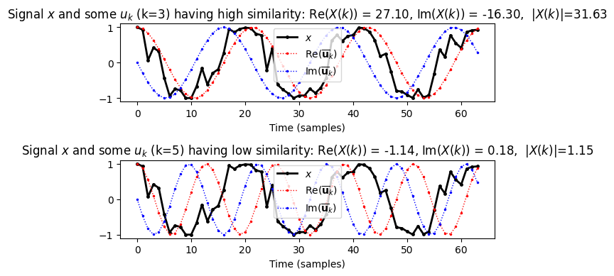
DFT 행렬 (DFT Matrix)
선형 연산자 \(\mathbb{C}^N \to \mathbb{C}^N\)이면, DFT는 \(N\times N\)-행렬로 표현할 수 있다. 이는 다음과 같은 유명한 DFT 행렬 \(\mathrm{DFT}_N \in \mathbb{C}^{N\times N}\) 행렬로 이어진다. \[\mathrm{DFT}_N(n, k) = \mathrm{exp}(-2 \pi i k n / N)\] for \(n\in[0:N-1]\) and \(k\in[0:N-1]\).
\(\rho_N:=\exp(2 \pi i / N)\)를 단위 N승근 (primitive Nth roots of unity)이라고 한다. 또한 단위 N승근을 다음과 같이 정의한다.
- \(\sigma_N:= \overline{\rho_N} = \mathrm{exp}(-2 \pi i / N)\)
지수 함수의 속성으로부터 다음을 얻을 수 있다.
- \(\sigma_N^{kn} = \mathrm{exp}(-2 \pi i / N)^{kn} = \mathrm{exp}(-2 \pi i k n / N)\)
이로부터 다음의 행렬을 얻는다. \[ \mathrm{DFT}_N = \begin{pmatrix} 1 & 1 & 1 & \dots & 1 \\ 1 & \sigma_N & \sigma_N^2 & \dots & \sigma_N^{N-1} \\ 1 & \sigma_N^2 & \sigma_N^4 & \dots & \sigma_N^{2(N-1)} \\ \vdots & \vdots & \vdots & \ddots & \vdots \\ 1 & \sigma_N^{N-1} & \sigma_N^{2(N-1)} & \dots & \sigma_N^{(N-1)(N-1)} \\ \end{pmatrix} \]
다음 그림에서 \(\mathrm{DFT}_N\)의 실수 및 허수 부분이 표시되며, 값은 적절한 색상으로 인코딩된다. \(\mathrm{DFT}_N\)의 \(k^\mathrm{th}\) 행은 위에 정의된 벡터 \(\mathbf{u}_k\)에 해당한다.
def generate_matrix_dft(N, K):
    """Generates a DFT (discrete Fourier transfrom) matrix

    Args:
        N (int): Number of samples
        K (int): Number of frequency bins

    Returns:
        dft (np.ndarray): The DFT matrix
    """
    dft = np.zeros((K, N), dtype=np.complex128)
    for n in range(N):
        for k in range(K):
            dft[k, n] = np.exp(-2j * np.pi * k * n / N)
    return dft

def dft(x):
    """Compute the disrcete Fourier transfrom (DFT)

    Args:
        x (np.ndarray): Signal to be transformed

    Returns:
        X (np.ndarray): Fourier transform of x
    """
    x = x.astype(np.complex128)
    N = len(x)
    dft_mat = generate_matrix_dft(N, N)
    return np.dot(dft_mat, x)
N = 32
dft_mat = generate_matrix_dft(N, N)
plt.figure(figsize=(10, 3))
plt.subplot(1, 2, 1)
plt.title('$\mathrm{Re}(\mathrm{DFT}_N)$')
plt.imshow(np.real(dft_mat), origin='lower', cmap='seismic', aspect='equal')
plt.xlabel('Time index $n$')
plt.ylabel('Frequency index $k$')
plt.colorbar()
plt.subplot(1, 2, 2)
plt.title('$\mathrm{Im}(\mathrm{DFT}_N)$')
plt.imshow(np.imag(dft_mat), origin='lower', cmap='seismic', aspect='equal')
plt.xlabel('Time index $n$')
plt.ylabel('Frequency index $k$')
plt.colorbar()
plt.tight_layout()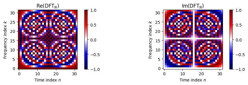
N = 128
n = np.arange(N)
k = 10
x = np.cos(2 * np.pi * (k * n / N) + 2 * (np.random.rand(N) - 0.5))
X = dft(x)

plt.figure(figsize=(8, 3))

plt.subplot(1, 2, 1)
plt.title('$x$')
plt.plot(x)
plt.xlabel('Time (index $n$)')

plt.subplot(1, 2, 2)
plt.title('$|X|$')
plt.plot(np.abs(X))
plt.xlabel('Frequency (index $k$)')
plt.tight_layout()
고속 푸리에 변환 (Fast Fourier Transform, FFT)
다음으로 DFT를 계산하는 빠른 알고리즘인 고속 푸리에 변환(FFT)에 대해 설명한다. FFT 알고리즘은 원래 1805년 즈음에 Gauss에 의해 발견되었고 1965년에 Cooley와 Tukey에 의해 재발견되었다.
FFT 알고리즘은 짝수 크기 \(N=2M\)의 DFT를 적용하는 것이 \(M\)의 절반 크기인 두 개의 DFT를 적용하는 것으로 표현될 수 있다는 관찰을 기반으로 한다. DFT 행렬의 \(\sigma_N^{kn} = \mathrm{exp}(-2 \pi i / N)^{kn}\) 항목 사이에 대수 관계가 있다는 사실을 이용한다.
\[\sigma_M = \sigma_N^2\]
FFT 알고리즘에서 \(x\)의 짝수-인덱스와 홀수-인덱스 항목의 DFT를 계산한다. \[\begin{align} (A(0), \dots, A(N/2-1)) &= \mathrm{DFT}_{N/2} \cdot (x(0), x(2), x(4), \dots, x(N-2))\\ (B(0), \dots, B(N/2-1)) &= \mathrm{DFT}_{N/2} \cdot (x(1), x(3), x(5), \dots, x(N-1)) \end{align}\]
\(N/2\) 크기의 두 DFT로 부터 \(N\) 크기의 전체 DFT를 다음과 같이 계산할 수 있다. \[ C(k) = \sigma_N^k \cdot B(k)\\ X(k) = A(k) + C(k)\\ X(N/2 + k) = A(k) - C(k) \] for \(k \in [0: N/2 - 1]\)
숫자 \(\sigma_N^k\)는 “twiddle factor”라고도 한다. \(N\)이 2의 거듭제곱인 경우, 이 아이디어는 \(\mathrm{DFT}_{1}\)(\(N=1\)의 경우)의 계산에 도달할 때까지 재귀적으로 적용될 수 있다.
def twiddle(N):
    """Generate the twiddle factors used in the computation of the fast Fourier transform (FFT)
    Args:
        N (int): Number of samples

    Returns:
        sigma (np.ndarray): The twiddle factors
    """
    k = np.arange(N // 2)
    sigma = np.exp(-2j * np.pi * k / N)
    return sigma


def fft(x):
    """Compute the fast Fourier transform (FFT)
    Args:
        x (np.ndarray): Signal to be transformed

    Returns:
        X (np.ndarray): Fourier transform of x
    """
    x = x.astype(np.complex128)
    N = len(x)
    log2N = np.log2(N)
    assert log2N == int(log2N), 'N must be a power of two!'
    X = np.zeros(N, dtype=np.complex128)

    if N == 1:
        return x
    else:
        this_range = np.arange(N)
        A = fft(x[this_range % 2 == 0])
        B = fft(x[this_range % 2 == 1])
        C = twiddle(N) * B
        X[:N//2] = A + C
        X[N//2:] = A - C
        return X
N = 16
n = np.arange(N)
k = 4
x = np.cos(2 * np.pi * (k * n / N) + 2 * (np.random.rand(N) - 0.5))
X_via_dft = dft(x)
X_via_fft = fft(x)
plt.figure(figsize=(8, 3))
plt.subplot(1, 2, 1)
plt.title('$x$')
plt.plot(x, marker='.', markersize=12)
plt.xlabel('Time (index $n$)')
plt.subplot(1, 2, 2)
plt.title('$|X|$')
plt.plot(np.abs(X_via_dft), marker='.', markersize=10, label='dft')
plt.plot(np.abs(X_via_fft), linestyle='--', color='pink', marker='.', markersize=6, label='fft')
plt.xlabel('Frequency (index $k$)')
plt.legend()
plt.tight_layout()
계산 복잡성
FFT는 전체 작업 수를 \(N^2\)(일반적인 행렬-벡터 곱 \(\mathrm{DFT}_N \cdot x\)를 계산할 때 필요함)에서 \(N\log_2N\) 정도로 줄인다. 예를 들어 \(N=2^{10}=1024\)를 사용하면 원래의 접근 방식의 \(N^2=1048576\) 작업 대신 FFT에 대략 \(N\log_2N=10240\)가 필요하다.
Python 코드의 작은 비트의 시간을 측정하는 간단한 방법을 제공하는
timeit모듈을 사용하여 실행 시간을 비교한다.
N = 512
n = np.arange(N)
x = np.sin(2 * np.pi * 5 * n / N )

print('Timing for DFT: ', end='')
%timeit dft(x)
print('Timing for FFT: ', end='')
%timeit fft(x)
Timing for DFT: 284 ms ± 6.98 ms per loop (mean ± std. dev. of 7 runs, 1 loop each)
Timing for FFT: 9.31 ms ± 216 µs per loop (mean ± std. dev. of 7 runs, 100 loops each)import timeit
Ns = [2 ** n for n in range(5, 11)]
times_dft = []
times_fft = []
execuctions = 5
for N in Ns:
n = np.arange(N)
x = np.sin(2 * np.pi * 5 * n / N )
time_dft = timeit.timeit(lambda: dft(x), number=execuctions) / execuctions
time_fft = timeit.timeit(lambda: fft(x), number=execuctions) / execuctions
times_dft.append(time_dft)
times_fft.append(time_fft)
plt.figure(figsize=(6, 3))
plt.plot(Ns, times_dft, '-xk', label='DFT')
plt.plot(Ns, times_fft, '-xr', label='FFT')
plt.xticks(Ns)
plt.legend()
plt.grid()
plt.xlabel('$N$')
plt.ylabel('Runtime (seconds)');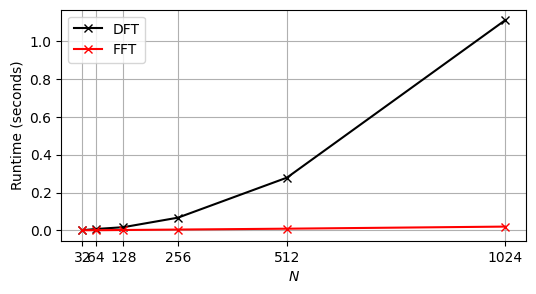
- FFT의 경우 계산이 훨씬 빠른 것을 볼 수 있다.
FFT 예시
- librosa
x, sr = librosa.load("../audio/c_strum.wav")
print(x.shape)
print(sr)
ipd.Audio(x, rate=sr)
(102400,)
22050X = scipy.fft.fft(x)
X_mag = np.absolute(X)
f = np.linspace(0, sr, len(X_mag)) # frequency variableplt.figure(figsize=(6, 2))
plt.plot(f, X_mag) # magnitude spectrum
plt.xlabel('Frequency (Hz)')
plt.show()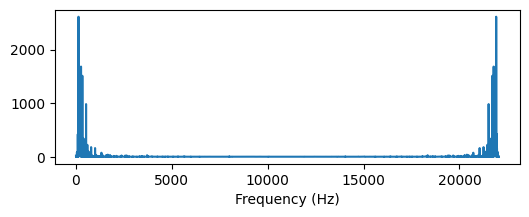
# zoom in
plt.figure(figsize=(6, 2))
plt.plot(f[:5000], X_mag[:5000])
plt.xlabel('Frequency (Hz)')
plt.show()
DFT - 위상(Phase)
- DFT 계산 결과, 복소 푸리에 계수가 나온다. 이 각 계수는 크기(magnitude) 및 위상(phase) 구성 요소로 나타낼 수 있다.
푸리에 계수의 극좌표 표현 (Polar Representation of Fourier Coefficients)
\(x=(x(0), x(1), ..., x(N-1))\)을 샘플 \(x(n)\in\mathbb{R}\) for \(n\in[0:N-1]\)을 가지는 시그널이라고 하자. 복소 푸리에 계수 \(c_k:=X(k)\in\mathbb{C}\) for \(k\in[0:N-1]\)는 DFT에 계산되어 다음과 같다. \[ c_k :=X(k) = \sum_{n=0}^{N-1} x(n) \exp(-2 \pi i k n / N). \]
\(c_k = a_k + i b_k\)를 실수부 \(a_k\in\mathbb{R}\)와 허수부 \(b_k\in\mathbb{R}\)로 구성된 복소수라고 할 때,
절대값은 \(|c_k| := \sqrt{a_k^2 + b_k^2}\)이고,
각도(래디안 단위)는 \(\gamma_k := \mathrm{angle}(c_k) := \mathrm{atan2}(b_k, a_k) \in [0,2\pi)\)이다.
지수 함수를 쓰면, 다음의 극좌표 표현을 얻는다. \[ c_k = |c_k| \cdot \mathrm{exp}(i \gamma_k). \]
최적화 Optimality 속성
\(\mathbf{cos}_{k,\varphi}:[0:N-1]\to\mathbb{R}\)를 주파수 파라미터 \(k\) 및 위상 \(\varphi\in[0 ,1)\)와 함께 샘플 정현파(sinusoid)라고 하면 다음과 같이 정의된다. \[ \mathbf{cos}_{k,\varphi}(n) = \sqrt{2}\mathrm{cos}\big( 2\pi (kn/N - \varphi) \big) \] for \(n\in[0,N-1]\)
직관적으로 말하자면, 길이 \(N\)의 이산 신호 \(x\)와 주파수 파라미터 \(k\)에 대한 푸리에 변환을 계산할 때 신호 \(x\)와 정현파 \(\mathbf{cos}_{k,\varphi_k}\)의 내적(일종의 상관 관계)을 계산한다.
\(\varphi_k\) 위상은 \(\varphi\in[0,1)\)로 \(x\)와 모든 가능한 정현파 \(\mathbf{cos}_{k,\varphi}\) 사이의 상관관계를 최대화한다는 속성을 가지고 있다.
\[ \varphi_k = \mathrm{argmax}_{\varphi\in[0,1)} \langle x | \mathbf{cos}_{k,\varphi} \rangle. \]
- 복소 푸리에 계수 \(X(k)\)는 기본적으로 복소수의 각도로 주어지는 이 최적 위상을 인코딩한다. 보다 정확하게 \(\gamma_k\)를 \(X(k)\)의 각도라고 하면, 최적 위상 \(\varphi_k\)가 다음과 같이 주어진다는 것을 알 수 있다.
\[ \varphi_k := - \frac{\gamma_k}{2 \pi}. \]
# Generate a chirp-like test signal (details not important)
N = 256
t_index = np.arange(N)
x = 1.8 * np.cos(2 * np.pi * (3 * (t_index * (1 + t_index / (4 * N))) / N))

k = 4
exponential = np.exp(-2 * np.pi * 1j * k * t_index / N)
X_k = np.sum(x * exponential)
phase_k = - np.angle(X_k) / (2 * np.pi)

def compute_plot_correlation(x, N, k, phase):
    sinusoid = np.cos(2 * np.pi * (k * t_index / N - phase))
    d_k = np.sum(x * sinusoid)
    plt.figure(figsize=(6,1.5))
    plt.plot(t_index, x, 'k')
    plt.plot(sinusoid, 'r')
    plt.title('Phase = %0.2f; correlation = %0.2f (optimal  = %0.2f)' % (phase, d_k, np.abs(X_k)))
    plt.tight_layout()
    plt.show()

print('Sinusoid with phase from Fourier coefficient resulting in an optimal correlation.')
compute_plot_correlation(x, N, k, phase=phase_k)

print('Sinusoid with an arbitrary phase resulting in a medium correlation.')
compute_plot_correlation(x, N, k, phase=0.4)

print('Sinusoid with a phase that yields a correlation close to zero.')
compute_plot_correlation(x, N, k, phase=0.51)
Sinusoid with phase from Fourier coefficient resulting in an optimal correlation.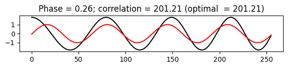
Sinusoid with an arbitrary phase resulting in a medium correlation.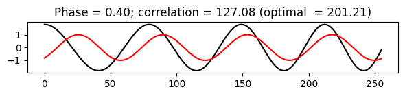
Sinusoid with a phase that yields a correlation close to zero.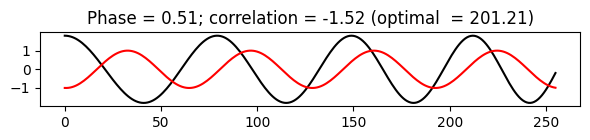
출처:
- https://www.audiolabs-erlangen.de/resources/MIR/FMP/C2/C2.html
\(\leftarrow\) 3.1. 복소수와 지수함수