3.4. 단기 푸리에 변환 (STFT) (2)

Short-Term Fourier Transform (2)

푸리에변환

STFT

Author

Cheonghyo Cho

Published

February 15, 2023

단기 푸리에 변환(SFTF)의 변형을 다룬다. 주파수 그리드 밀도(density), 보간법(interpolation), 그리고 역(inverse) 푸리에 변환 등을 소개한다.

이 글은 FMP(Fundamentals of Music Processing) Notebooks을 참고로 합니다.

import numpy as np
import matplotlib.pyplot as plt
import librosa
import librosa.display
import IPython.display as ipd
from scipy.interpolate import interp1d
import scipy

주파수 그리드 밀도 (Frequency Grid Density)

이산 STFT를 계산할 때 해상도(resolution)가 신호의 샘플링 레이트와 STFT 윈도우 크기에 따라 달라지는 주파수 그리드(frequency grid)가 있다. STFT 계산에서 윈도우가 있는 섹션을 적절하게 패딩(padding)하여 주파수 그리드를 더 조밀하게 만드는 방법에 대해 설명한다. 주파수 해상도란 원하는 신호를 주파수 도메인에서 관찰할 때 얼마나 촘촘한 간격으로 해당 주파수 대역의 값을 관찰 할 수 있는가를 말한다.

DFT 주파수 그리드

\(x\in \mathbb{R}^N\) 를 길이 \(N\in\mathbb{N}\)의 샘플 \(x(0), x(1), \ldots, x(N-1)\)의 이산 신호라고 하자.
샘플링 레이트 \(F_\mathrm{s}\)가 주어졌을 때, \(x\)는 연속 시간 신호 \(f:\mathbb{R}\to\mathbb{R}\)를 샘플링하여 얻는다고 가정한다.
그러면 이산 푸리에 변환(DFT) \(X := \mathrm{DFT}_N \cdot x\)은 특정 주파수에 대한 연속 푸리에 변환 \(\hat{f}\)의 근사치로 해석될 수 있다. \[ X(k) := \sum_{n=0}^{N-1} x(n) \exp(-2 \pi i k n / N) \approx {F_\mathrm{s}} \cdot \hat{f} \left(k \cdot \frac{F_\mathrm{s}}{N}\right) \] for \(k\in[0:N-1]\).
따라서 \(X(k)\)의 인덱스 \(k\)는 다음의 물리적 주파수(헤르츠단위)에 해당된다. \[\begin{equation} F_\mathrm{coef}^N(k) := \frac{k\cdot F_\mathrm{s}}{N} \end{equation}\]
즉, 이산 푸리에 변환은 \(\mathrm{DFT}_N\)의 크기 \(N\)에 따라 달라지는, 해상도 \(F_\mathrm{s}/N\)의 선형 주파수 그리드(frequency grid)를 얻는다.
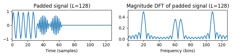
주파수 그리드의 밀도를 높이기 위한 한 가지 아이디어는 인위적으로 신호에 0을 추가하여 DFT의 크기를 늘리는 것이다.
이를 위해 \(L\in\mathbb{N}\) with \(L\geq N\)라고 하자. 그런 다음 \(\tilde{x}\in \mathbb{R}^L\) 신호를 얻기 위해 \(x\) 신호 오른쪽에 제로 패딩(zero padding)을 적용한다.

\[\tilde{x}(n) :=\left\{\begin{array}{ll} x(n) , \,\,\mbox{for}\,\, n \in[0:N-1]\\ 0, \,\,\mbox{for}\,\, n \in[N:L-1] \end{array}\right.\]

\(\mathrm{DFT}_L\)을 적용하면 다음을 얻는다. \[ \tilde{X}(k) = \mathrm{DFT}_L \cdot \tilde{x} = \sum_{n=0}^{L-1} \tilde{x}(n) \exp(-2 \pi i k n / L) = \sum_{n=0}^{N-1} x(n) \exp(-2 \pi i k n / L) \approx {F_\mathrm{s}} \cdot \hat{f} \left(k \cdot \frac{F_\mathrm{s}}{L}\right) \] for \(k\in[0:L-1]\).
이제 계수 \(\tilde{X}(k)\)는 다음의 물리적 주파수에 대응된다. \[\begin{equation} F_\mathrm{coef}^L(k) := \frac{k\cdot F_\mathrm{s}}{L}, \end{equation}\]
이는 선형 주파수 해상도 \(F_\mathrm{s}/L\)를 보인다.
예를 들어, \(L=2N\)인 경우 주파수 그리드 해상도는 2배 증가한다. 즉, DFT가 길수록 간격이 더 가까운 주파수 빈(bin)이 더 많아진다.
그러나 이 트릭은 DFT의 근사 품질을 개선하지 않는다는 점에 유의해야 한다(리만(Riemann) 근사의 합계 수는 여전히 \(N\)임에 유의하자).
단, \(L\geq N\) 및 제로 패딩을 사용할 때 주파수 축의 선형 샘플링이 정제(refine)된다.
다음 예는 \(\mathrm{DFT}_N \cdot x\)를 \(\mathrm{DFT}_L \cdot \tilde{x}\)와 비교한다.

Fs = 32
duration = 2
freq1 = 5
freq2 = 15
N = int(duration * Fs)
t = np.arange(N) / Fs
t1 = t[:N//2]
t2 = t[N//2:]

x1 = 1.0 * np.sin(2 * np.pi * freq1 * t1)
x2 = 0.7 * np.sin(2 * np.pi * freq2 * t2)
x = np.concatenate((x1, x2))

plt.figure(figsize=(8, 2))

ax1 = plt.subplot(1, 2, 1)
plt.plot(x)
plt.title('Orginal signal ($N$=%d)' % N)
plt.xlabel('Time (samples)')
plt.xlim([0, N - 1])
plt.subplot(1, 2, 2)
Y = np.abs(np.fft.fft(x)) / Fs
plt.plot(Y)
plt.title('Magnitude DFT of original signal ($N$=%d)' % N)
plt.xlabel('Frequency (bins)')
plt.xlim([0, N - 1])
plt.tight_layout()

L = 2 * N
pad_len = L - N
t_tilde = np.concatenate((t, np.arange(len(x), len(x) + pad_len) / Fs))
x_tilde = np.concatenate((x, np.zeros(pad_len)))
                         
plt.figure(figsize=(8, 2))
ax1 = plt.subplot(1, 2, 1)
plt.plot(x_tilde)
plt.title('Padded signal ($L$=%d)' % L)
plt.xlabel('Time (samples)')
plt.xlim([0, L - 1])
plt.subplot(1, 2, 2)
Y_tilde = np.abs(np.fft.fft(x_tilde)) / Fs
plt.plot(Y_tilde)
plt.title('Magnitude DFT of padded signal ($L$=%d)' % L)
plt.xlabel('Frequency (bins)')
plt.xlim([0, L - 1])

plt.tight_layout()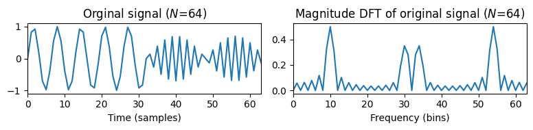

다음 코드 예제는 증가된 주파수 그리드 해상도로 DFT를 계산하는 함수를 구현한다.
여기에서 모든 파라미터는 물리적 방식으로 해석된다(초 및 헤르츠 기준).

def compute_plot_DFT_extended(t, x, Fs, L):
    N = len(x)
    pad_len = L - N
    t_tilde = np.concatenate((t, np.arange(len(x), len(x) + pad_len) / Fs))
    x_tilde = np.concatenate((x, np.zeros(pad_len)))
    Y = np.abs(np.fft.fft(x_tilde)) / Fs    
    Y = Y[:L//2]
    freq = np.arange(L//2)*Fs/L
    # freq = np.fft.fftfreq(L, d=1/Fs)
    # freq = freq[:L//2]
    plt.figure(figsize=(10, 2))
    
    ax1 = plt.subplot(1, 3, 1)
    plt.plot(t_tilde, x_tilde)
    plt.title('Signal ($N$=%d)' % N)
    plt.xlabel('Time (seconds)')
    plt.xlim([t[0], t[-1]])
    
    ax2 = plt.subplot(1, 3, 2)
    plt.plot(t_tilde, x_tilde)
    plt.title('Padded signal (of size $L$=%d)' % L)
    plt.xlabel('Time (seconds)')
    plt.xlim([t_tilde[0], t_tilde[-1]])    
    
    ax3 = plt.subplot(1, 3, 3)
    plt.plot(freq, Y)
    plt.title('Magnitude DFT of padded signal ($L$=%d)' % L)
    plt.xlabel('Frequency (Hz)')
    plt.xlim([freq[0], freq[-1]])
    plt.tight_layout()           

    return ax1, ax2, ax3

N = len(x)

L = N
ax1, ax2, ax3 = compute_plot_DFT_extended(t, x, Fs, L)

L = 2 * N
ax1, ax2, ax3 = compute_plot_DFT_extended(t, x, Fs, L)

L = 4 * N
ax1, ax2, ax3 = compute_plot_DFT_extended(t, x, Fs, L)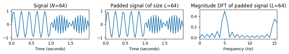

주파수 그리드 해상도가 증가된 STFT

이제 동일한 제로-패딩 전략을 사용하여 STFT의 주파수 그리드 해상도를 높이는 방법을 보자. librosa 함수 librosa.stft는 두 개의 파라미터 n_fft(\(L\)에 해당) 및 win_length(\(N\)에 해당)를 통해 이 아이디어를 구현한다. 파라미터를 물리적 도메인으로 변환할 때 주의해야 한다.
바이올린이 연주하는 음 C4의 예를 보자

x, Fs = librosa.load("../audio/violin_c4_legato.wav")
ipd.display(ipd.Audio(x, rate=Fs))

t_wav = np.arange(0, x.shape[0]) * 1 / Fs
plt.figure(figsize=(5, 1.5))
plt.plot(t_wav, x, c='gray')
plt.xlim([t_wav[0], t_wav[-1]])
plt.xlabel('Time (seconds)')
plt.tight_layout()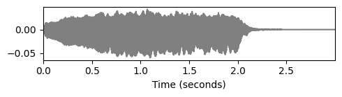

이제 제로 패딩으로 STFT를 계산한다. 그림에서 축은 시간 프레임 및 주파수 빈으로 표시된다.

def compute_stft(x, Fs, N, H, L=N, pad_mode='constant', center=True):    
    X = librosa.stft(x, n_fft=L, hop_length=H, win_length=N, 
                     window='hann', pad_mode=pad_mode, center=center)
    Y = np.log(1 + 100 * np.abs(X) ** 2)
    F_coef = librosa.fft_frequencies(sr=Fs, n_fft=L)
    T_coef = librosa.frames_to_time(np.arange(X.shape[1]), sr=Fs, hop_length=H) 
    return Y, F_coef, T_coef

def plot_compute_spectrogram(x, Fs, N, H, L, color='gray_r'):
    Y, F_coef, T_coef = compute_stft(x, Fs, N, H, L)
    plt.imshow(Y, cmap=color, aspect='auto', origin='lower')
    plt.xlabel('Time (frames)')
    plt.ylabel('Frequency (bins)')
    plt.title('L=%d' % L)
    plt.colorbar()

N = 256
H = 64
color = 'gray_r' 
plt.figure(figsize=(8, 3))

L = N
plt.subplot(1,3,1)
plot_compute_spectrogram(x, Fs, N, H, L)

L = 2 * N
plt.subplot(1,3,2)
plot_compute_spectrogram(x, Fs, N, H, L)

L = 4 * N
plt.subplot(1,3,3)
plot_compute_spectrogram(x, Fs, N, H, L)

plt.tight_layout()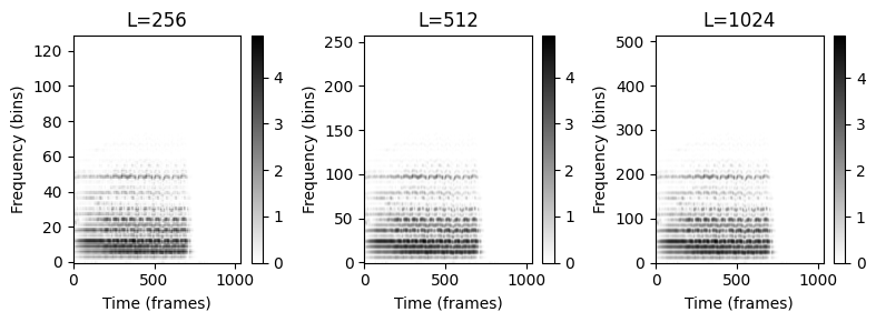

다음으로 동일한 계산을 반복한다. 여기서 축은 이제 초와 헤르츠로 지정된 물리적 단위를 표시하도록 변환된다. 또한 시간-주파수 평면을 확대하여 밀도가 높은 주파수 그리드 밀도의 효과를 강조한다.

def plot_compute_spectrogram_physical(x, Fs, N, H, L, xlim, ylim, color='gray_r'):
    Y, F_coef, T_coef = compute_stft(x, Fs, N, H, L)
    extent=[T_coef[0], T_coef[-1], F_coef[0], F_coef[-1]]
    plt.imshow(Y, cmap=color, aspect='auto', origin='lower', extent=extent)
    plt.xlabel('Time (seconds)')
    plt.ylabel('Frequency (Hz)')
    plt.title('L=%d' % L)
    plt.ylim(ylim)
    plt.xlim(xlim)
    plt.colorbar()

xlim_sec = [1, 2]
ylim_hz = [2000, 3000]

plt.figure(figsize=(8, 3))

L = N
plt.subplot(1,3,1)
plot_compute_spectrogram_physical(x, Fs, N, H, L, xlim=xlim_sec, ylim=ylim_hz)

L = 2 * N
plt.subplot(1,3,2)
plot_compute_spectrogram_physical(x, Fs, N, H, L, xlim=xlim_sec, ylim=ylim_hz)

L = 4 * N
plt.subplot(1,3,3)
plot_compute_spectrogram_physical(x, Fs, N, H, L, xlim=xlim_sec, ylim=ylim_hz)

plt.tight_layout()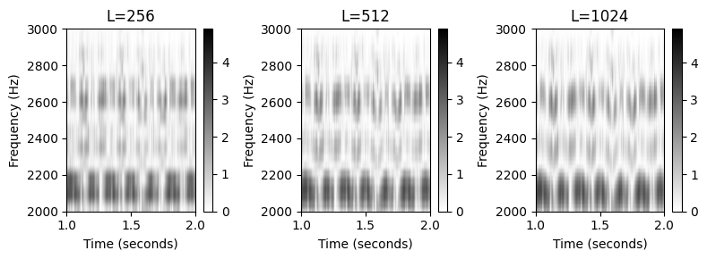

librosa 함수 librosa.stft는 두 개의 파라미터 n_fft(패딩된 섹션의 크기 \(L\)에 해당) 및 win_length(\(N\)에 해당, 윈도우 부분)가 있다. 이 패딩 변형을 \(L\)(\(N\) 대신)와 함께 사용하면, 함수 \(F_\mathrm{coef}\)의 계산을 다음과 같이 조정해야 한다. \[\begin{equation} F_\mathrm{coef}(k) := \frac{k\cdot F_\mathrm{s}}{L} \end{equation}\] for \(k\in [0:K]\) with \(K=L/2\).
반올림 문제를 방지하려면 짝수 \(L\)(아마도 2의 거듭제곱)를 선택하는 것이 좋다.

N = 256
L = 512
H = 64
color = 'gray_r' 

X = librosa.stft(x, n_fft=L, hop_length=H, win_length=N, window='hann', pad_mode='constant', center=True) # center에 대해서는 밑에서 다루기로 한다
Y = np.log(1 + 100 * np.abs(X) ** 2)

T_coef = np.arange(0, X.shape[1]) * H / Fs

K = L // 2
F_coef = np.arange(K + 1) * Fs / L # 공식에 따라
F_coef_librosa = librosa.fft_frequencies(sr=Fs, n_fft=L) # librosa 내장
print('F_coef 결과가 같은가:', np.allclose(F_coef, F_coef_librosa))
print('Y.shape = (%d,%d)'%(Y.shape[0],Y.shape[1]))

plt.figure(figsize=(6, 3))
extent = [T_coef[0], T_coef[-1], F_coef[0], F_coef[-1]]
plt.imshow(Y, cmap=color, aspect='auto', origin='lower', extent=extent)
plt.xlabel('Time (seconds)')
plt.ylabel('Frequency (Hz)')
plt.colorbar()
plt.tight_layout()

F_coef 결과가 같은가: True
Y.shape = (257,1034)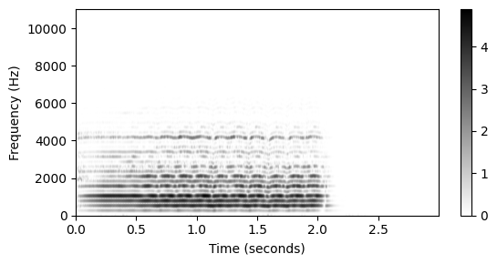

주파수 그리드 보간법 (Frequency Grid Interpolation)

위에서는 STFT 계산에서 윈도우 섹션을 적절하게 패딩하여 밀도를 높이는 방법을 보았다.
대안으로 주파수 해상도를 조정하기 위해 주파수 방향을 따른 보간법(interpolation) 기술에 대해 논의한다.

보간법 (Interpolation)

데이터 포인트 시퀀스가 주어지면 보간법 interpolation의 목표는 의미 있는 방식으로 시퀀스를 정제(refine)하는 중간(intermediate) 데이터 포인트를 계산하는 것이다.
보다 구체적으로, 파라미터 \(t\in\mathbb{R}\)를 \(f(t)\in\mathbb{R}\)로 매핑하는 \(f\colon\mathbb{R}\to\mathbb{R}\) 함수를 고려해보자.
\(n\in\mathbb{Z}\)에 대한 파라미터 \(t_n\in\mathbb{R}\)의 이산 집합에 대해서만 \(f(t_n)\) 값이 있다고 가정하자. \(t_{n} > t_ {n-1}\).
그런 다음 보간법의 목표는 \(f^\ast(t)\) 값을 추정하는 것이다. \(f(t_n)\)는 다음과 같이 주어진다.

\[f^\ast(t) \approx f(t)\] for any \(t\in\mathbb{R}\)

실제로는 \(f\) 함수는 알 수 없지만, 종종 \(f\)의 연속성, 평활성, 미분 가능성 등과 같은 특정 속성을 가정한다.
가장 간단한 보간법 방법은 조각 상수 보간(piecewise constant interpolation)(또는 최근접 이웃(nearest neighbor) 보간법)이다. 파라미터 \(t\in\mathbb{R}\)가 주어지면, 가장 가까운 파라미터 \(t_n\)을 취하여 다음을 정의한다.
- \(f^\ast(t)=f(t_n).\)

# Simulates the original function
t = np.arange(-0.5, 10.5, 0.01)
f = np.sin(2 * t)

# Known funcion values
t_n = np.arange(0, 11)
f_n = np.sin(2 * t_n)

# Interpolation
f_interpol_nearest = interp1d(t_n, f_n, kind='nearest', fill_value='extrapolate')(t)

plt.figure(figsize=(8, 2)) 
plt.plot(t, f, color=(0.8, 0.8, 0.8))
plt.plot(t, f_interpol_nearest, 'r-')
plt.plot(t_n, f_n, 'ko')
plt.ylim([-1.5,1.5])
plt.title('Piecewise constant interpolation')
plt.tight_layout()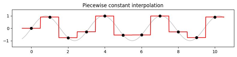

최근접 이웃 보간법은 일반적으로 이산 함수를 생성한다. 연속적인 보간법 함수를 얻기 위한 간단한 대안으로는 선형 보간법(linear interpolation)이 있다.
\(t_{n-1}\)와 \(t_n\) 사이에 있는 파라미터 \(t\)가 주어지면, 다음과 같이 정의할 수 있다. \[ f^\ast(t)=f(t_{n-1}) + (f(t_{n})-f(t_{n-1}))\cdot\frac{t-t_{n-1}}{t_{n} - t_{n-1}}. \]

f_interpol_linear = interp1d(t_n, f_n, kind='linear', fill_value='extrapolate')(t)

plt.figure(figsize=(8, 2)) 
plt.plot(t, f, color=(0.8, 0.8, 0.8))
plt.plot(t, f_interpol_linear, 'r-')
plt.plot(t_n, f_n, 'ko')
plt.ylim([-1.5,1.5])
plt.title('Linear interpolation')
plt.tight_layout()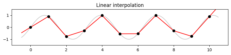

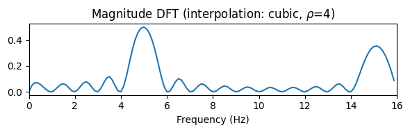
Python 클래스 scipy.inperploate.interp1d는 Nearest-neighbor, 선형 및 다양한 차수의 spline 보간을 포함하여 여러 종류의 보간 방법을 제공한다. 또 다른 예로, 3차 보간(3차 스플라인)에 대한 결과를 보자.

f_interpol_cubic = interp1d(t_n, f_n, kind='cubic', fill_value='extrapolate')(t)

plt.figure(figsize=(8, 2)) 
plt.plot(t, f, color=(0.8, 0.8, 0.8))
plt.plot(t, f_interpol_cubic, 'r-')
plt.plot(t_n, f_n, 'ko')
plt.ylim([-1.5,1.5])
plt.title('Cubic interpolation')
plt.tight_layout()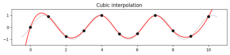

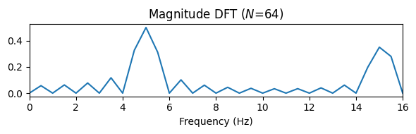
주파수 보간법

선형 주파수 그리드의 밀도를 증가시키기 위해 제로 패딩을 기반으로 더 큰 DFT를 사용할 수 있었다. 이제 주파수 영역에서 보간법을 적용하여 대안을 소개한다.
\(x\in \mathbb{R}^N\)를 길이 \(N\in\mathbb{N}\), 샘플링 레이트 \(F_\mathrm{s}\), DFT \(X = \mathrm{DFT} _N \cdot x\), 및 DFT 크기 \(Y=|X|\)의 이산 신호라고 하자. 그러면 \(Y(k)\)의 인덱스 \(k\)는 다음의 헤르츠로 주어진 물리적 주파수에 해당한다.

\[\begin{equation} F_\mathrm{coef}(k) := \frac{k\cdot F_\mathrm{s}}{N} \end{equation}\]

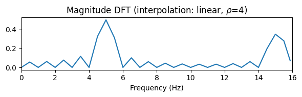
즉, 주파수 그리드 결과의 해상도는 \(F_\mathrm{s}/N\)이다. 팩터 \(\rho\in\mathbb{N}\)를 도입하여, 해상도 \(F_\mathrm{s}/(\rho\cdot N)\)를 고려하여 주파수 그리드를 정제(refine)한다. 이 주파수 그리드를 기반으로 보간 기술을 사용하여 크기 주파수 계수(magnitude frequency coefficient)를 계산한다.

Fs = 32
duration = 2
omega1 = 5
omega2 = 15
N = int(duration * Fs)
t = np.arange(N) / Fs
t1 = t[:N//2]
t2 = t[N//2:]

x1 = 1.0 * np.sin(2 * np.pi * omega1 * t1)
x2 = 0.7 * np.sin(2 * np.pi * omega2 * t2)
x = np.concatenate((x1, x2))

plt.figure(figsize=(6, 2))
plt.plot(t, x)
plt.title('Orginal signal ($N$=%d)' % N)
plt.xlabel('Time (seconds)')
plt.xlim([t[0], t[-1]])   
plt.tight_layout()

Y = np.abs(np.fft.fft(x)) / Fs
Y = Y[:N//2+1]
F_coef = np.arange(N//2+1)*Fs/N
plt.figure(figsize=(6, 2))
plt.plot(F_coef,Y)
plt.title('Magnitude DFT ($N$=%d)' % N)
plt.xlabel('Frequency (Hz)')
plt.xlim([F_coef[0], F_coef[-1]])     
plt.tight_layout()

def interpolate_plot_DFT(N, Fs, F_coef, rho, int_method):
    F_coef_interpol = np.arange(F_coef[0], F_coef[-1], Fs/(rho*N))
    Y_interpol = interp1d(F_coef, Y, kind=int_method)(F_coef_interpol)
    plt.figure(figsize=(6, 2))
    plt.plot(F_coef_interpol, Y_interpol)
    plt.title(r'Magnitude DFT (interpolation: %s, $\rho$=%d)'%(int_method,rho))
    plt.xlabel('Frequency (Hz)')
    plt.xlim([F_coef[0], F_coef[-1]])
    plt.tight_layout()

rho = 4
interpolate_plot_DFT(N=N, Fs=Fs, F_coef=F_coef, rho=rho, int_method='nearest')
interpolate_plot_DFT(N=N, Fs=Fs, F_coef=F_coef, rho=rho, int_method='linear')
interpolate_plot_DFT(N=N, Fs=Fs, F_coef=F_coef, rho=rho, int_method='cubic')

STFT를 위한 보간법

STFT의 주파수 그리드를 정제하기 위해서 주파수 방향을 따라 보간법을 적용할 수 있다.
이전과 같은 바이올린(C4)의 예로 보자.

x, Fs = librosa.load("../audio/violin_c4_legato.wav")
ipd.display(ipd.Audio(x, rate=Fs))

t_wav = np.arange(0, x.shape[0]) * 1 / Fs
plt.figure(figsize=(6, 1))
plt.plot(t_wav, x, c='gray')
plt.xlim([t_wav[0], t_wav[-1]])
plt.xlabel('Time (seconds)');

def stft_convention_fmp(x, Fs, N, H, pad_mode='constant', center=True, mag=False, gamma=0):
    """Compute the discrete short-time Fourier transform (STFT)

    Args:
        x (np.ndarray): Signal to be transformed
        Fs (scalar): Sampling rate
        N (int): Window size
        H (int): Hopsize
        pad_mode (str): Padding strategy is used in librosa (Default value = 'constant')
        center (bool): Centric view as used in librosa (Default value = True)
        mag (bool): Computes magnitude STFT if mag==True (Default value = False)
        gamma (float): Constant for logarithmic compression (only applied when mag==True) (Default value = 0)

    Returns:
        X (np.ndarray): Discrete (magnitude) short-time Fourier transform
    """
    X = librosa.stft(x, n_fft=N, hop_length=H, win_length=N,
                     window='hann', pad_mode=pad_mode, center=center)
    if mag:
        X = np.abs(X)**2
        if gamma > 0:
            X = np.log(1 + gamma * X)
    F_coef = librosa.fft_frequencies(sr=Fs, n_fft=N)
    T_coef = librosa.frames_to_time(np.arange(X.shape[1]), sr=Fs, hop_length=H)
    # T_coef = np.arange(X.shape[1]) * H/Fs
    # F_coef = np.arange(N//2+1) * Fs/N
    return X, T_coef, F_coef


def compute_f_coef_linear(N, Fs, rho=1):
    """Refines the frequency vector by factor of rho

    Args:
        N (int): Window size
        Fs (scalar): Sampling rate
        rho (int): Factor for refinement (Default value = 1)

    Returns:
        F_coef_new (np.ndarray): Refined frequency vector
    """
    L = rho * N
    F_coef_new = np.arange(0, L//2+1) * Fs / L
    return F_coef_new


def interpolate_freq_stft(Y, F_coef, F_coef_new):
    """Interpolation of STFT along frequency axis

    Args:
        Y (np.ndarray): Magnitude STFT
        F_coef (np.ndarray): Vector of frequency values
        F_coef_new (np.ndarray): Vector of new frequency values

    Returns:
        Y_interpol (np.ndarray): Interploated magnitude STFT
    """
    compute_Y_interpol = interp1d(F_coef, Y, kind='cubic', axis=0)
    Y_interpol = compute_Y_interpol(F_coef_new)
    return Y_interpol


def plot_compute_spectrogram_physical(x, Fs, N, H, xlim, ylim, rho=1, color='gray_r'):
    Y, T_coef, F_coef = stft_convention_fmp(x, Fs, N, H, mag=True, gamma=100)
    F_coef_new = compute_f_coef_linear(N, Fs, rho=rho)
    Y_interpol = interpolate_freq_stft(Y, F_coef, F_coef_new)    
    extent=[T_coef[0], T_coef[-1], F_coef[0], F_coef[-1]]
    plt.imshow(Y_interpol, cmap=color, aspect='auto', origin='lower', extent=extent)
    plt.xlabel('Time (seconds)')
    plt.ylabel('Frequency (Hz)')
    plt.title(r'$\rho$=%d' % rho)
    plt.ylim(ylim)
    plt.xlim(xlim)
    plt.colorbar()

xlim_sec = [1, 2]
ylim_hz = [2000, 3000]

N = 256
H = 64
plt.figure(figsize=(10, 4))
 
plt.subplot(1, 3, 1)
plot_compute_spectrogram_physical(x, Fs, N, H, xlim=xlim_sec, ylim=ylim_hz, rho=1)

plt.subplot(1, 3, 2)
plot_compute_spectrogram_physical(x, Fs, N, H, xlim=xlim_sec, ylim=ylim_hz, rho=2)

plt.subplot(1, 3, 3)
plot_compute_spectrogram_physical(x, Fs, N, H, xlim=xlim_sec, ylim=ylim_hz, rho=4)

plt.tight_layout()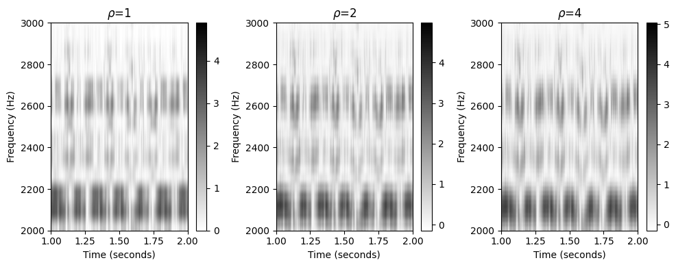

로그-주파수 STFT

이 보간법은 주파수 그리드의 비선형 변형에 사용될 수 있다. 예를 들어 선형 간격의 주파수 축(헤르츠로 측정)을 로그 간격의 주파수 축(피치 또는 센트로 측정)으로 변환할 수 있다.
로그 간격의 주파수 그리드를 정의하는 것이 주요 단계이다. 이때 음정에 사용되는 대수 측정 단위인 센트라는 개념을 사용한다. 참조 주파수 \(\omega_0\)가 주어지면 임의의 주파수 \(\omega\)와 \(\omega_0\) 사이의 거리는 다음과 같이 지정된다. \[ \log_2\left(\frac{\omega}{\omega_0}\right)\cdot 1200 \]
다음 함수에서는 최소 주파수 값(매개변수 F_min이 기준 주파수 \(\omega_0\)로 사용되므로 \(0\) cents에 해당함)에서 시작하여 로그 간격의 주파수 축을 계산한다.
또한 이 함수에는 로그 해상도를 센트 단위로 지정하는 파라미터 R이 있다. 즉, 로그 주파수 축에서 두 개의 연속된 주파수 빈은 R 센트 떨어져 있다.
최대 주파수는 다른 매개변수 F_max에 의해 지정된다.
다음 예에서 주파수 F_min = 100(\(0\) 센트에 해당) 및 F_max = 3200(\(6000\) 센트에 해당)을 사용한다. 또한 해상도는 R=20(옥타브당 \(60\) 주파수 빈에 해당)으로 설정한다.

def compute_f_coef_log(R, F_min, F_max):
    """Adapts the frequency vector in a logarithmic fashion

    Args:
        R (scalar): Resolution (cents)
        F_min (float): Minimum frequency
        F_max (float): Maximum frequency (not included)

    Returns:
        F_coef_log (np.ndarray): Refined frequency vector with values given in Hz)
        F_coef_cents (np.ndarray): Refined frequency vector with values given in cents.
            Note: F_min serves as reference (0 cents)
    """
    n_bins = np.ceil(1200 * np.log2(F_max / F_min) / R).astype(int)
    F_coef_log = 2 ** (np.arange(0, n_bins) * R / 1200) * F_min
    F_coef_cents = 1200 * np.log2(F_coef_log / F_min)
    return F_coef_log, F_coef_cents

N = 1024
H = 256
Y, T_coef, F_coef = stft_convention_fmp(x, Fs, N, H, mag=True, gamma=100)

F_min = 100
F_max = 3200
R = 20
F_coef_log, F_coef_cents = compute_f_coef_log(R, F_min, F_max)

print('#bins=%3d, F_coef[0]      =%6.2f, F_coef[1]      =%6.2f, F_coef[-1]      =%6.2f'%(len(F_coef),F_coef[0], F_coef[1], F_coef[-1]))
print('#bins=%3d, F_coef_log[0]  =%6.2f, F_coef_log[1]  =%6.2f, F_coef_log[-1]  =%6.2f'%(len(F_coef_log),F_coef_log[0], F_coef_log[1], F_coef_log[-1]))
print('#bins=%3d, F_coef_cents[0]=%6.2f, F_coef_cents[1]=%6.2f, F_coef_cents[-1]=%6.2f'%(len(F_coef_cents),F_coef_cents[0], F_coef_cents[1], F_coef_cents[-1]))

#bins=513, F_coef[0]      =  0.00, F_coef[1]      = 21.53, F_coef[-1]      =11025.00
#bins=300, F_coef_log[0]  =100.00, F_coef_log[1]  =101.16, F_coef_log[-1]  =3163.24
#bins=300, F_coef_cents[0]=  0.00, F_coef_cents[1]= 20.00, F_coef_cents[-1]=5980.00

Y_interpol = interpolate_freq_stft(Y, F_coef, F_coef_log)
color = 'gray_r' 

plt.figure(figsize=(10, 4))
plt.subplot(1, 3, 1)
extent=[T_coef[0], T_coef[-1], F_coef[0], F_coef[-1]]
plt.imshow(Y, cmap=color, aspect='auto', origin='lower', extent=extent)
y_ticks_freq = np.array([100, 400, 800, 1200, 1600, 2000, 2400, 2800, 3200])
plt.yticks(y_ticks_freq)
plt.xlabel('Time (seconds)')
plt.ylabel('Frequency (Hz)')
plt.title('Linear frequency axis')
plt.ylim([F_min, F_max])
plt.colorbar()

plt.subplot(1, 3, 2)
extent=[T_coef[0], T_coef[-1], F_coef_cents[0], F_coef_cents[-1]]
plt.imshow(Y_interpol, cmap=color, aspect='auto', origin='lower', extent=extent)
y_tick_freq_cents = 1200 * np.log2(y_ticks_freq / F_min)
plt.yticks(y_tick_freq_cents, y_ticks_freq)
plt.xlabel('Time (seconds)')
plt.ylabel('Frequency (Hz)')
plt.title('Log-frequency axis')
plt.title('Log-frequency axis with R=%d' % R)
plt.colorbar()

plt.subplot(1, 3, 3)
extent=[T_coef[0], T_coef[-1], F_coef_cents[0], F_coef_cents[-1]]
plt.imshow(Y_interpol, cmap=color, aspect='auto', origin='lower', extent=extent)
y_ticks_cents = np.array([0, 1200, 2400, 3600, 4800, 6000])
plt.yticks(y_ticks_cents)
plt.xlabel('Time (seconds)')
plt.ylabel('Frequency (cents)')
plt.title('Log-frequency axis')
plt.title('Log-frequency axis with R=%d' % R)
plt.colorbar()
plt.tight_layout()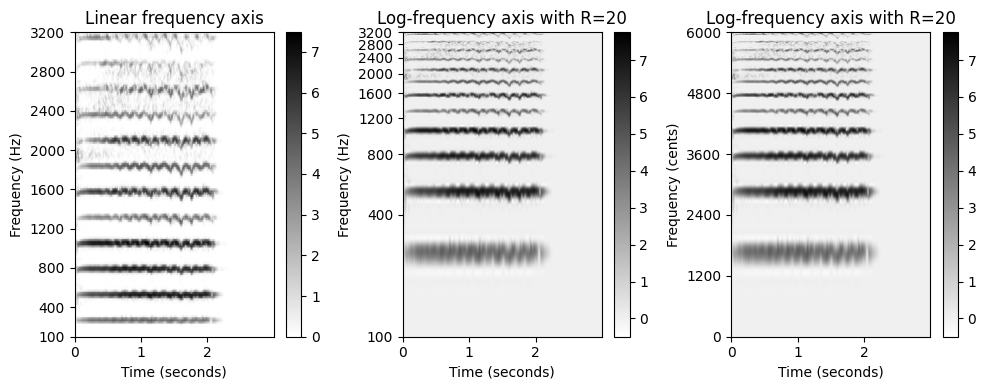

STFT: Conventions and Implementations

샘플 신호에 대한 시간 축

\(x=(x(0),x(1), \ldots x(L-1))^\top \in \mathbb{R}^L\)을 길이가 \(L\in\mathbb{N}\)인 이산-시간 신호라고 가정하자. 또한 \(F_\mathrm{s}\)를 샘플 레이트라고 하자.
그런 다음 물리적 시간 위치(초 단위로 표시)의 벡터 \(t=(t(0),t(1), \ldots t(L-1))^\top \in \mathbb{R}^L\)을 \(x\)에 대입하면 다음과 같이 정의된다. \[ t(n) = \frac{n}{F_\mathrm{s}} \] for \(n\in[0:L-1]\)
다시 말해,
- 샘플 \(x(0)\)는 물리적 시간 \(t(0)=0\)(초 단위로 표시됨)와 연관된다.
- 신호 \(x\)의 기간(duration)(초 단위)은 샘플 수를 샘플링 속도로 나눈 것이다: \(L/F_\mathrm{s}\). 단, 이것은 \(t(L-1)=(L-1)/F_\mathrm{s}\)와 동일하지 않다.
- 두 샘플 \(x(n-1)\) 및 \(x(n)\) 사이의 거리(샘플링 기간 sampling period이라고 함)는 \(1/F_\mathrm{s}\)이다.

x, Fs = librosa.load("../audio/violin_c4_legato.wav")
ipd.Audio(x, rate=Fs)
L = x.shape[0] #샘플 수
t_wav = np.arange(L) / Fs
x_duration = L / Fs #듀레이션

print('t[0] = %0.4f, t[-1] = (L-1)/Fs = %0.4f, Fs = %0.0f, L = %0.0f, dur_x=%0.4f'
      % (t_wav[0], t_wav[-1], Fs, L, x_duration))
ipd.display(ipd.Audio(x, rate=Fs))

plt.figure(figsize=(6, 2))
plt.plot(t_wav, x, color='gray')
plt.xlim([t_wav[0], t_wav[-1]])
plt.xlabel('Time (seconds)')
plt.tight_layout()

t[0] = 0.0000, t[-1] = (L-1)/Fs = 3.0000, Fs = 22050, L = 66150, dur_x=3.0000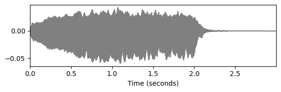

# librosa를 이용한 plot
# 단 librosa는 파형의 샘플이 아닌 symmetric amplitude envelope를 그림

plt.figure(figsize=(6, 2))
librosa.display.waveshow(x, color='gray')
plt.tight_layout()

중심 윈도우잉과 시간 변환 (Centered Windowing and Time Conversion)

신호의 윈도우 부분을 고려할 때 중앙 (centered) 시점을 채택한다. 여기서 윈도우의 중심이란 물리적 도메인과 관련된 참조로 사용된다.
특히 STFT를 계산할 때, 윈도우 길이의 절반의 제로-패딩을 적용하여 신호를 왼쪽으로 확장한다.
보다 정확히 말하면, \(w:[0:N-1]\to\mathbb{R}\)를 짝수 윈도우 길이 \(N\in\mathbb{N}\)의 윈도우 함수라고 하고 \(H\in\mathbb{ N}\)를 홉(hop) 크기라고 하자. 그리고 \(N/2\)개 0값을 앞에 넣는다.

\[ \tilde{x}=(0,\ldots,0,x(0),x(1), \ldots x(L-1))^\top \in \mathbb{R}^{L+N/2} \]

\[ \mathcal{X}(m,k):= \sum_{n=0}^{N-1} \tilde{x}(n+mH)w(n)\mathrm{exp}(-2\pi ikn/N). \]

또한 프레임 인덱스 \(m\)이 물리적 시간 위치와 연관되어 있는 규칙을 사용한다.
- \(T_\mathrm{coef}(m) := \frac{m\cdot H}{F_\mathrm{s}}\)
특히 다음이 성립한다.
- 프레임 인덱스 \(m=0\)는 물리적 시간 \(T_\mathrm{coef}(0)=0\)(초 단위)에 해당한다.
- 시간 해상도(즉, 연속되는 두 프레임 사이의 거리)은 \(\Delta t = H/F_\mathrm{s}\)(초 단위)이다.

주파수 변환 (Frequency Conversion)

\(x\) 및 \(w\)가 실수이면 주파수 계수의 상위 절반이 중복된다. 따라서 계수 \(k\in[0:K]\) (\(K=N/2\))만 사용된다.
특히 인덱스 \(k=N/2\)는 나이퀴스트(Nyquist) 주파수 \(\omega=F_\mathrm{s}/2\)에 해당한다.
또한 인덱스 \(k\)는 다음의 주파수에 해당한다(헤르츠 단위).
- \(F_\mathrm{coef}(k) := \frac{k\cdot F_\mathrm{s}}{N}\)

스펙트로그램 시각화

다음 코드는 이러한 규칙을 구현하기 위해 librosa 함수 librosa.stft를 사용하는 방법을 보여준다. 파라미터 설정 center=True는 centered view를 활성화하고 pad_mode='constant'는 제로-패딩 모드로 전환한다.
또한 이 코드는 변환 함수 \(T_\mathrm{coef}\) 및 \(F_\mathrm{coef}\)를 한 번은 위의 공식을 사용하고 한 번은 librosa 내장 함수를 사용하여 구현하는 방법을 보여준다. 홀수 윈도우 크기 \(N\)의 경우 반올림에 대한 다른 규칙이 있을 수 있다. 실제로는 일반적으로 짝수 윈도우 크기를 사용한다(특히 FFT algorithm 관점에서 2의 거듭제곱임).

N = 256
H = 64
color = 'gray_r' 

X = librosa.stft(x, n_fft=N, hop_length=H, win_length=N, window='hann', pad_mode='constant', center=True)
Y = np.log(1 + 100 * np.abs(X) ** 2)

T_coef = np.arange(X.shape[1]) * H / Fs #위의 공식
T_coef_librosa = librosa.frames_to_time(np.arange(X.shape[1]), sr=Fs, hop_length=H) #librosa 내장
print('T_coef 계산 결과가 같은가:', np.allclose(T_coef, T_coef_librosa))

K = N // 2
F_coef = np.arange(K+1) * Fs / N #위의 공식
F_coef_librosa = librosa.fft_frequencies(sr=Fs, n_fft=N) #librosa 내장
print('F_coef 계산 결과가 같은가:', np.allclose(F_coef, F_coef_librosa))

plt.figure(figsize=(6, 3))
extent = [T_coef[0], T_coef[-1], F_coef[0], F_coef[-1]]
plt.imshow(Y, cmap=color, aspect='auto', origin='lower', extent=extent)
plt.xlabel('Time (seconds)')
plt.ylabel('Frequency (Hz)')
plt.colorbar()
plt.tight_layout()
plt.show()

T_coef 계산 결과가 같은가: True
F_coef 계산 결과가 같은가: True

시각화에서 centered view를 채택하려면 프레임 길이의 절반만큼 왼쪽 및 오른쪽 여백을 조정하고, 빈(bin) 너비의 절반만큼 아래쪽 및 위쪽 여백을 조정해야 한다.
그러나 큰 스펙트로그램의 경우 시각화의 이러한 작은 조정은 상관 없다.

plt.figure(figsize=(6, 3))
extent = [T_coef[0] - (H / 2) / Fs, T_coef[-1] + (H / 2) / Fs,
          F_coef[0] - (Fs / N) / 2, F_coef[-1] + (Fs / N) / 2]
plt.imshow(Y, cmap=color, aspect='auto', origin='lower', extent=extent)
plt.xlim([T_coef[0], T_coef[-1]])
plt.ylim([F_coef[0], F_coef[-1]])
plt.xlabel('Time (seconds)')
plt.ylabel('Frequency (Hz)')
plt.colorbar()
plt.tight_layout()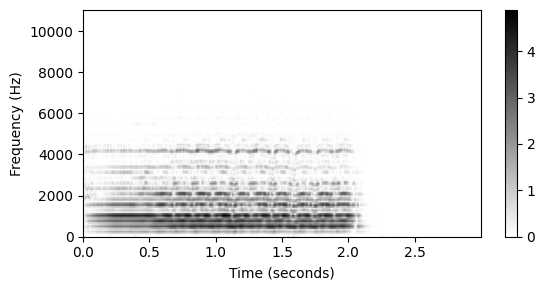

# librosa의 내장 함수로 결과를 비교하자

plt.figure(figsize=(6, 3))
librosa.display.specshow(Y, y_axis='linear', x_axis='time', sr=Fs, hop_length=H, cmap=color)
plt.colorbar()
plt.tight_layout()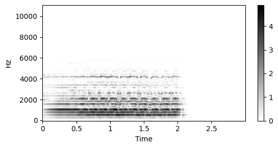

역 푸리에 변형 (Inverse Fourier Transform)

역(Inverse) DFT

\(N\in\mathbb{N}\) 길이의 벡터 \(x\in \mathbb{C}^N\)가 주어지면 DFT은 행렬-벡터 곱으로 정의된다. \[X = \mathrm{DFT}_N \cdot x\]
- with \(\mathrm{DFT}_N \in \mathbb{C}^{N\times N}\)
- given by \(\mathrm{DFT}_N(n, k) = \mathrm{exp}(-2 \pi i k n / N)\)
- for \(n\in[0:N-1]\) and \(k\in[0:N-1]\).
DFT는 벡터 \(x\)를 스펙트럼 벡터 \(X\)에서 복구할 수 있다는 점에서 invertible하다. 역 DFT는 행렬-벡터 곱으로 다시 지정된다. \[ x = \mathrm{DFT}_N^{-1} \cdot X, \]
여기서 \(\mathrm{DFT}_N^{-1}\)는 DFT 행렬 \(\mathrm{DFT}_N\)의 역을 나타낸다.
- \(\mathrm{DFT}_N^{-1}(n, k) = \frac{1}{N}\mathrm{exp}(2 \pi i k n / N)\)
- for \(n\in[0:N-1]\) and \(k\in[0:N-1]\).
즉, 역함수는 본질적으로 일부 정규화 인자(normalizing factor) 및 켤레 복소수(complex conjugation)까지 DFT 행렬과 일치한다.
다음 코드 셀에서 DFT 행렬과 그 역행렬을 생성한다. 또한 두 행렬이 실제로 서로 역임을 보여준다.
- 이를 위해 \(\mathrm{DFT}_N \cdot \mathrm{DFT}_N^{-1}\)와 항등 행렬 \(I_N\in \mathbb{R}^{N\times N}\)의 차이, 그리고 \(\mathrm{DFT}_N^{-1} \cdot\mathrm{DFT}_N\)와 \(I_N\)의 차이를 측정한다.

def generate_matrix_dft(N, K):
    """Generates a DFT (discrete Fourier transfrom) matrix
    Args:
        N (int): Number of samples
        K (int): Number of frequency bins
    Returns:
        dft (np.ndarray): The DFT matrix
    """
    dft = np.zeros((K, N), dtype=np.complex128)
    for n in range(N):
        for k in range(K):
            dft[k, n] = np.exp(-2j * np.pi * k * n / N)
    return dft

def generate_matrix_dft_inv(N, K):
    """Generates an IDFT (inverse discrete Fourier transfrom) matrix
    Args:
        N (int): Number of samples
        K (int): Number of frequency bins
    Returns:
        dft (np.ndarray): The IDFT matrix
    """
    dft = np.zeros((K, N), dtype=np.complex128)
    for n in range(N):
        for k in range(K):
            dft[k, n] = np.exp(2j * np.pi * k * n / N) / N
    return dft

N = 32
dft_mat = generate_matrix_dft(N, N)
dft_mat_inv = generate_matrix_dft_inv(N, N)

I = np.eye(N)
A =  np.dot(dft_mat, dft_mat_inv)
B =  np.dot(dft_mat_inv, dft_mat)

plt.figure(figsize=(11, 3))

plt.subplot(1, 3, 1)
plt.title(r'$I_N$ for $N = %d$'%N)
plt.imshow(I, origin='lower', cmap='seismic', aspect='equal')
plt.colorbar()

plt.subplot(1, 3, 2)
plt.title(r'$|I_N - \mathrm{DFT}_N \cdot \mathrm{DFT}_N^{-1}|$')
plt.imshow(np.abs(I-A), origin='lower', cmap='seismic', aspect='equal')
plt.colorbar()

plt.subplot(1, 3, 3)
plt.title(r'$|I_N - \mathrm{DFT}_N^{-1} \cdot \mathrm{DFT}_N|$')
plt.imshow(np.abs(I-B), origin='lower', cmap='seismic', aspect='equal')
plt.colorbar();

plt.tight_layout()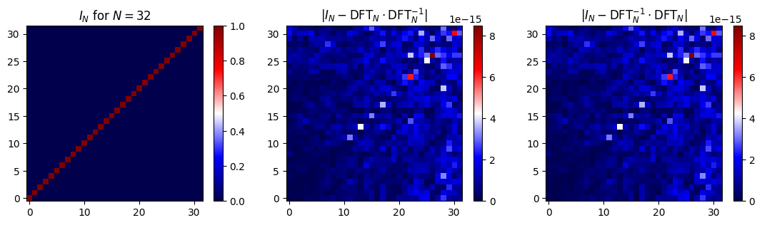

DFT는 FFT 알고리즘을 사용하여 효율적으로 계산할 수 있다. 역 DFT 계산에도 적용할 수 있다. 다음에서는 numpy.fft.fft 및 numpy.fft.ifft를 사용해 구현한다.

역(Inverse) STFT

다음으로 이산 STFT을 inverting하는 법을 보자.
\(x:\mathbb{Z}\to\mathbb{R}\)를 이산-시간 신호라고 하고, \(\mathcal{X}\)를 그것의 STFT라고 하자.
또한 \(w:[0:N-1]\to\mathbb{R}\)를 길이 \(N\in\mathbb{N}\) 및 홉 크기 파라미터 \(H\in\mathbb{N}\)의 실수 값 이산 윈도우 함수를 나타낸다고 하자.
표기상 편의를 위해 제로-패딩을 사용하여 윈도우 함수를 \(w:\mathbb{Z}\to\mathbb{R}\)로 확장한다.
\(x_n:\mathbb{Z}\to\mathbb{R}\)를 다음에 의해 정의된 윈도우 신호라고 하자.
- \(x_n(r):=x(r+nH)w(r)\) for \(r\in\mathbb{Z}\).
그러면 STFT 계수 \(\mathcal{X}(n,k)\) for \(k\in[0:N-1]\)가 다음에 의해 얻어진다.
- \((\mathcal{X}(n,0),\ldots, \mathcal{X}(n,N-1))^\top = \mathrm{DFT}_N \cdot (x_n(0),\ldots, x_n(N-1))^\top.\)
\(\mathrm{DFT}_N\)가 invertible 행렬이기 때문에 STFT에서의 윈도우 신호 \(x_n\)를 다음과 같이 재구성할 수 있다. \[(x_n(0),\ldots x_n(N-1))^\top = \mathrm{DFT}_N^{-1} \cdot (\mathcal{X}(n,0),\ldots, \mathcal{X}(n,N-1))^\top\]
원래 신호의 샘플 \(x(r)\)을 얻으려면 윈도우 프로세스를 반대로 해야 한다. 이것은 윈도우 프로세스에서 상대적으로 약한 조건에서 가능하다는 것을 볼 수 있다. 신호의 윈도우 섹션의 적절하게 이동된 모든 버전에 대한 중첩(superposition)을 고려해 보자. \[\sum_{n\in\mathbb{Z}} x_n(r-nH) = \sum_{n\in\mathbb{Z}} x(r-nH+nH)w(r-nH) = x(r)\sum_{n\in\mathbb{Z}} w(r-nH)\]
따라서 샘플 \(x(r)\)를 다음을 통해 복구할 수 있다. \[x(r) = \frac{\sum_{n\in\mathbb{Z}} x_n(r-nH)}{\sum_{n\in\mathbb{Z}} w(r-nH)}\]
- \(\sum_{n\in\mathbb{Z}} w(r-nH)\not= 0\)
이 전반적인 접근 방식은 소위 overlap–add technique을 기반으로 한다. 이 기술에서는 겹치는 재구성된 윈도우 섹션이 단순히 오버레이되고 합산된다(그런 다음 windowing을 보상하기 위해 정규화됨).

단위 분할 (Partition of Unity)

위의 조건을 만족하는 홉 크기와 함께 윈도우 함수를 찾는 것은 어렵지 않다. 예를 들어 윈도우 함수 \(w:[0:N-1]\to\mathbb{R}\)가 양수이고 홉 크기가 윈도우 길이보다 작거나 같을 때 time-shifted 윈도우에 대한 합계는 항상 양수이다.
종종 윈도우 함수와 홉 크기를 다음의 더 강한 조건으로 선택할 수도 있다.
- \(\sum_{n\in\mathbb{Z}} w(r-nH) = 1\) (for all \(r\in\mathbb{Z}\) is fulfilled.)
이 경우, time-shifted 윈도우 함수는 이산 시간 축 \(\mathbb{Z}\)의 단위 분할 (partition of unity)을 정의한다고 한다.
예를 들어, 다음과 같이 정의된 윈도우 \(w:\mathbb{Z}\to\mathbb{R}\)로 squared sinusoidal을 사용할 때 단위 분할을 얻는다.
- \(w(r):= \left\{ \begin{array}{cl} \sin(\pi r/N)^2 \quad \mbox{if}\,\,\, r\in[0:N-1] \\ 0 \quad \mbox{otherwise} \end{array} \right.\)
- 홉 사이즈는 \(H=N/2\)
단위 분할이 되는 속성은 윈도우 함수 자체뿐만 아니라 홉 크기 파라미터에도 의존한다는 점에 유의해야 한다.
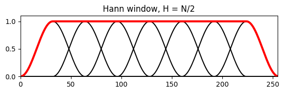
다음 그림은 \(N\) 길이의 다양한 윈도우 함수와 홉 크기 \(H\)를 사용하는 time-shifted 버전을 보여준다. time-shifted 버전의 합은 두꺼운 빨간색 곡선으로 표시된다.

def plot_sum_window(w, H, L, title='', figsize=(6, 2)):
    N = len(w)
    M = np.floor((L - N) / H).astype(int) + 1
    w_sum = np.zeros(L)
    plt.figure(figsize=figsize)
    for m in range(M):
        w_shifted = np.zeros(L)
        w_shifted[m * H:m * H + N] = w
        plt.plot(w_shifted, 'k')
        w_sum = w_sum + w_shifted
    plt.plot(w_sum, 'r', linewidth=3)
    plt.xlim([0, L-1])
    plt.ylim([0, 1.1*np.max(w_sum)])
    plt.title(title)
    plt.tight_layout()
    plt.show()
    return w_sum

L = 256
N = 64

H = N//2
w_type = 'triang'
w = scipy.signal.get_window(w_type, N)
plot_sum_window(w, H, L, title='Triangular window, H = N/2');

H = N//2
w_type = 'hann'
w = scipy.signal.get_window(w_type, N)
plot_sum_window(w, H, L, title='Hann window, H = N/2');

H = 3*N//8
w_type = 'hann'
w = scipy.signal.get_window(w_type, N)
plot_sum_window(w, H, L, title='Hann window, H = 3N/8');

H = N//4
w = scipy.signal.gaussian(N, std=8)
plot_sum_window(w, H, L, title='Gaussian window, H = N/4');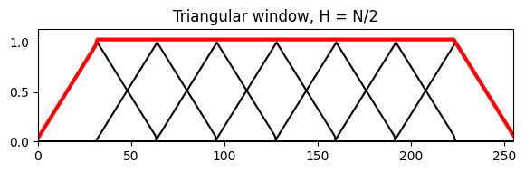

구현

역 DFT에서 작은 허수값을 피하기 위해 재구성된 윈도우 신호의 실수 부분만 유지하는게 이득일 수 있다.
역 DFT를 적용한 후에는 윈도잉을 보상해야 한다. 프레임 기반 레벨에서(즉, 각 윈도우 섹션에 대해 개별적으로) 이 작업을 수행하는 것 보다는 모든 윈도우 신호와 이동된 모든 윈도우를 개별적으로 누적하여 전역적으로(globally) 보상을 수행해야 한다. 전역 보상이 가능한 이유는 DFT의 선형성에 있다. 또한 보상에서 0으로 나누기를 피해야 한다.
주어진 홉 크기에 대해 이동된 윈도우가 단위 분할(a partition of unity)을 형성하는 경우, 보상을 수행할 필요가 없다.
STFT 계산에서 패딩이 적용된 경우 역 STFT 계산 시 이를 고려해야 한다.

def stft_basic(x, w, H=8, only_positive_frequencies=False):
    """Compute a basic version of the discrete short-time Fourier transform (STFT)
    Args:
        x (np.ndarray): Signal to be transformed
        w (np.ndarray): Window function
        H (int): Hopsize (Default value = 8)
        only_positive_frequencies (bool): Return only positive frequency part of spectrum (non-invertible)
            (Default value = False)
    Returns:
        X (np.ndarray): The discrete short-time Fourier transform
    """
    N = len(w)
    L = len(x)
    M = np.floor((L - N) / H).astype(int) + 1
    X = np.zeros((N, M), dtype='complex')
    for m in range(M):
        x_win = x[m * H:m * H + N] * w
        X_win = np.fft.fft(x_win)
        X[:, m] = X_win

    if only_positive_frequencies:
        K = 1 + N // 2
        X = X[0:K, :]
    return X

def istft_basic(X, w, H, L):
    """Compute the inverse of the basic discrete short-time Fourier transform (ISTFT)
    Args:
        X (np.ndarray): The discrete short-time Fourier transform
        w (np.ndarray): Window function
        H (int): Hopsize
        L (int): Length of time signal
    Returns:
        x (np.ndarray): Time signal
    """
    N = len(w)
    M = X.shape[1]
    x_win_sum = np.zeros(L)
    w_sum = np.zeros(L)
    for m in range(M):
        x_win = np.fft.ifft(X[:, m])
        # Avoid imaginary values (due to floating point arithmetic)
        x_win = np.real(x_win)
        x_win_sum[m * H:m * H + N] = x_win_sum[m * H:m * H + N] + x_win
        w_shifted = np.zeros(L)
        w_shifted[m * H:m * H + N] = w
        w_sum = w_sum + w_shifted
    # Avoid division by zero
    w_sum[w_sum == 0] = np.finfo(np.float32).eps
    x_rec = x_win_sum / w_sum
    return x_rec, x_win_sum, w_sum

L = 256
t = np.arange(L) / L
omega = 4
x = np.sin(2 * np.pi * omega * t * t)

N = 64
H = 3 * N // 8
w_type = 'hann'
w = scipy.signal.get_window(w_type, N)
X = stft_basic(x, w=w, H=H)
x_rec, x_win_sum, w_sum = istft_basic(X, w=w, H=H, L=L)

plt.figure(figsize=(8, 3))
plt.plot(x, color=[0, 0, 0], linewidth=4, label='Original signal')
plt.plot(x_win_sum, 'b', label='Summed windowed signals')
plt.plot(w_sum, 'r', label='Summed windows')
plt.plot(x_rec, color=[0.8, 0.8, 0.8], linestyle=':', linewidth=4, label='Reconstructed signal')
plt.xlim([0,L-1])
plt.legend(loc='lower left')
plt.tight_layout()
plt.show()

librosa 예제

단, librosa.istft에서는 다른 윈도우 보상 방법을 사용한다. \[x(r) = \frac{\sum_{n\in\mathbb{Z}} w(r-nH)x_n(r-nH)}{\sum_{n\in\mathbb{Z}} w(r-nH)^2}\]

def print_plot(x, x_rec):
    print('Number of samples of x:    ', x.shape[0])
    print('Number of samples of x_rec:', x_rec.shape[0])
    if x.shape[0] == x_rec.shape[0]:
        print('Signals x and x_inv agree:', np.allclose(x, x_rec))
        plt.figure(figsize=(6, 2))
        plt.plot(x-x_rec, color='red')
        plt.xlim([0, x.shape[0]])
        plt.title('Differences between x and x_rec')
        plt.xlabel('Time (samples)');
        plt.tight_layout()
        plt.show()
    else:
        print('Number of samples of x and x_rec does not agree.')

x, Fs = librosa.load("../audio/violin_c4_legato.wav")        
        
N = 4096
H = 2048
L = x.shape[0]

print('=== Centered Case ===')
X = librosa.stft(x, n_fft=N, hop_length=H, win_length=N, window='hann', pad_mode='constant', center=True)
x_rec = librosa.istft(X, hop_length=H, win_length=N, window='hann', center=True, length=L)
print('stft: center=True; istft: center=True')
print_plot(x, x_rec)

print('=== Non-Centered Case ===')
X = librosa.stft(x, n_fft=N, hop_length=H, win_length=N, window='hann', pad_mode='constant', center=False)
x_rec = librosa.istft(X, hop_length=H, win_length=N, window='hann', center=False, length=L)
print('stft: center=False; istft: center=False')
print_plot(x, x_rec)

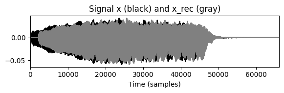
print('=== Centered vs. Non-Centered Case ===')
X = librosa.stft(x, n_fft=N, hop_length=H, win_length=N, window='hann', pad_mode='constant', center=True)
x_rec = librosa.istft(X, hop_length=H, win_length=N, window='hann', center=False, length=L)
print('stft: center=True; istft: center=False')
print_plot(x, x_rec)

plt.figure(figsize=(6, 2))
plt.plot(x, color='black')
plt.xlim([0, x.shape[0]])
plt.plot(x_rec, color='gray')
plt.title('Signal x (black) and x_rec (gray)')
plt.xlabel('Time (samples)');
plt.tight_layout()
plt.show()

=== Centered Case ===
stft: center=True; istft: center=True
Number of samples of x:     66150
Number of samples of x_rec: 66150
Signals x and x_inv agree: True

=== Non-Centered Case ===
stft: center=False; istft: center=False
Number of samples of x:     66150
Number of samples of x_rec: 66150
Signals x and x_inv agree: False

=== Centered vs. Non-Centered Case ===
stft: center=True; istft: center=False
Number of samples of x:     66150
Number of samples of x_rec: 66150
Signals x and x_inv agree: False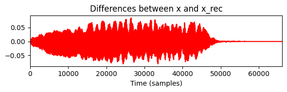

출처:

https://www.audiolabs-erlangen.de/resources/MIR/FMP/C2/C2.html
https://musicinformationretrieval.com/

구글 Colab 링크

\(\leftarrow\) 3.3. 단기 푸리에 변환 (STFT) (1)

3.5. 디지털 신호 \(\rightarrow\)