import IPython.display as ipd
import librosa
import librosa.display
import numpy as np; import pandas as pd
import matplotlib.pyplot as plt
import matplotlib.gridspec as gridspec
from scipy import signal
from scipy.interpolate import interp1d
from utils.plot_tools import plot_chromagram, plot_matrix, plot_segments, plot_signal, plot_segments_overlay
from utils.feature_tools import smooth_downsample_feature_sequence, normalize_feature_sequence5.1. 음악 구조와 분할
Music Structure and Segmentation
음악구조분석
분할
크로마그램
MFCC
템포그램
주어진 음악 녹음에 대한 구조적(structural) 분석과 시간적 분할(segmentation)를 소개하고, 반복성(repitition), 동질성(homogeneity) 및 새로움(novelty)을 기반으로 하는 기본 분할 원칙에 대해 논의한다.
이 글은 FMP(Fundamentals of Music Processing) Notebooks을 참고로 합니다.
음악 구조 분석의 일반 원칙
- 음악 구조 분석(music structure analysis)은 다양한 측면에 의존하는 다면적이고 정의가 모호한 문제이다.
- 우선 문제의 복잡성은 분석할 음악 표현의 종류에 따라 다르다. 예를 들어 악보에서 반복되는 멜로디와 같은 특정 구조를 감지하는 것은 비교적 쉬운 반면, 오디오 표현에서는 어렵다.
- 둘째, 분할(segmentation)의 기반이 될 수 있는 동질성, 반복, 새로움 등 다양한 원칙이 있다.
- 셋째, 멜로디, 하모니, 리듬 또는 음색과 같은 다양한 음악적 차원을 설명해야 한다. 마지막으로 분할(segmentation)과 구조(structure)는 음악적 맥락과 고려해야 할 시간적 계층(temporal hierarchy) 에 따라 크게 달라진다.
- 다음 그림은 음악 구조를 다룰 때 고려해야 할 다양한 측면에 대한 개요를 제공한다.
ipd.Image("../img/5.music_structure_analysis/FMP_C4_F02.png", width=600)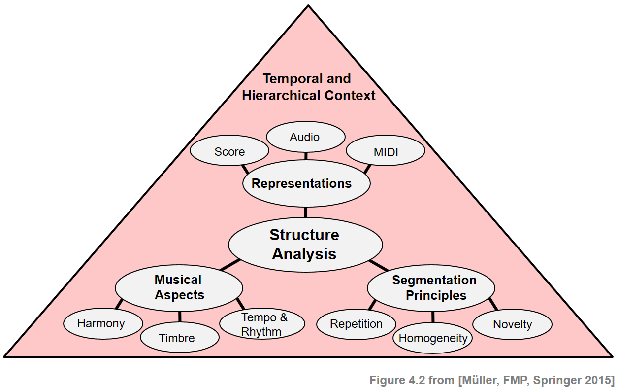
분할과 구조 분석 (Segmentation and Structure Analysis)
분할/세분화(Segmentation) 은 일반적으로 원본보다 더 의미 있고 분석하기 쉬운 것으로 표시를 단순화하기 위해 지정된 문서를 여러 세그먼트로 분할하는 과정을 말한다. 예를 들어 이미지 처리에서 목표는 주어진 이미지를 영역 집합으로 분할하여 각 영역이 색상, 강도 또는 질감과 같은 일부 특성과 관련하여 유사하도록 하는 것이다. 영역 경계는 종종 이미지 밝기 또는 기타 속성이 급격하게 변하고 불연속성을 나타내는 등고선이나 가장자리로 설명될 수 있다.
음악에서 분할 작업은 주어진 오디오 스트림을 음향적으로 의미 있는 섹션으로 분해하는 것이다. 각각은 시작 및 종료 경계(boundary) 로 지정된 연속 시간 간격에 해당한다.
미세한 수준에서의 분할은 개별 음 사이의 경계를 찾거나 비트 위치에 의해 지정된 비트 간격을 찾는 것을 목표로 할 수 있다. 대략적인 수준에서의 목표는 악기나 화음의 변화를 감지하거나 절(verse)과 합창 부분 사이의 경계를 찾는 것일 수 있다. 또한 침묵, 말, 음악을 구별하거나 실제 음악 녹음의 시작 부분을 찾거나 공연이 끝난 후 박수를 분리하는 것이 전형적인 분할 작업이다.
구조 분석(structural analysis) 의 목표는 단순한 분할을 넘어 세그먼트 간의 관계를 찾고 이해하는 것이다.
예를 들어, 특정 세그먼트는 악기에 의해 특징지어질 수 있다. 현악기로만 연주되는 구간이 있을 수 있으며, 전체 오케스트라가 연주하는 섹션 다음에 솔로 섹션이 이어질 수 있다. 노래하는 목소리가 있는 절 부분은 순전히 기악 부분으로 대체될 수 있다. 또는 부드럽고 느린 도입부 부분이 훨씬 빠른 템포로 연주되는 메인 테마 앞에 나올 수 있다.
또한 섹션이 자주 반복된다. 대부분의 음악 관련 이벤트는 어떤 식으로든 반복된다. 그러나 반복은 원래 섹션과 거의 동일하지 않으며 가사, 악기 또는 멜로디와 같은 측면에서 조금씩 수정된다. 구조 분석의 주요 작업 중 하나는 주어진 음악 녹음을 분할하는 것뿐만 아니라 세그먼트를 음악적으로 의미 있는 범주(예: 인트로, 코러스, 절, 아웃트로)로 그룹화하는 것이다.
전산 음악 구조 분석의 문제는 음악의 구조가 반복, 대조, 변형 및 동질성을 비롯한 다양한 종류의 관계에서 발생한다는 것이다. 음악 구조에 결정적으로 영향을 미치는 다양한 원리를 고려하여 음악 구조 분석에 대한 다양한 접근 방식이 많이 개발되었다. 세 가지 방법 분류를 대략적으로 구분해보자.
- 첫째, 반복(repetition) 기반 방법은 반복 패턴을 식별하는 데 사용된다.
- 둘째, 새로움(novelty) 기반 방법을 사용하여 대조되는 부분 간의 전환을 감지한다.
- 셋째, 동질성(homogeneity) 기반 방법은 일부 음악적 속성과 관련하여 일관된 구절을 결정하는 데 사용된다.
새로움 기반 및 동질성 기반 접근 방식은 동전의 양면 같다. 새로움 감지는 더 동질적인 세그먼트 이후의 놀라운 이벤트 또는 변화를 관찰하는 것을 기반으로 한다. 새로움 감지의 목적은 변경 사항의 시간 위치를 찾는 것이지만 동질성 분석의 초점은 일부 음악적 속성과 관련하여 일관성 있는 더 긴 악절을 식별하는 데 있다.
다음 그림은 유사한 분할 및 구조화 원칙이 이미지 및 3D 데이터와 같은 다른 도메인에 적용됨을 보여준다.
ipd.Image("../img/5.music_structure_analysis/FMP_C4_F03_text.png", width=600)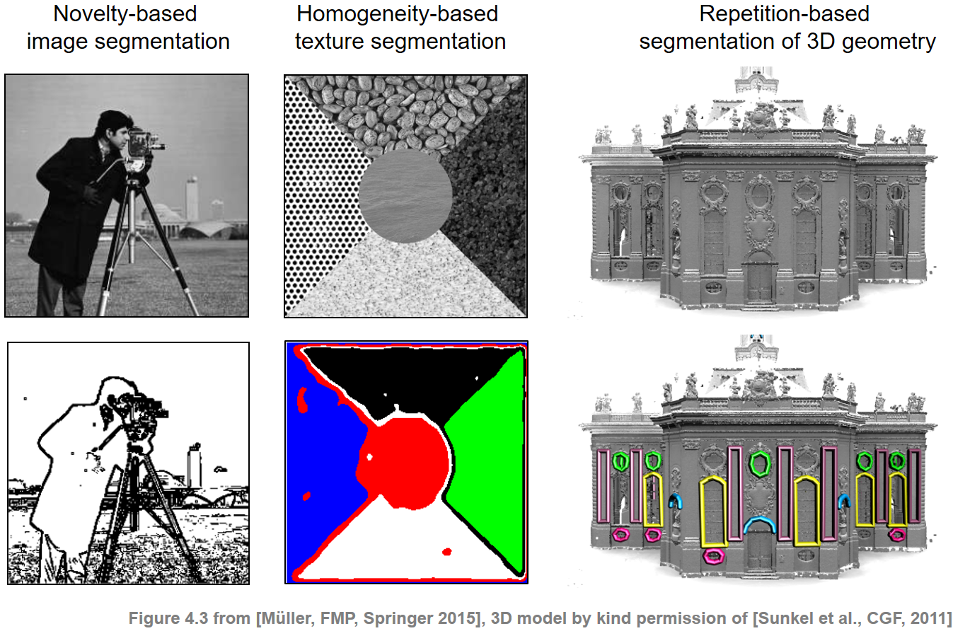
음악 구조 (Musical Structure)
- 음악 구조를 구체화하기 위해 몇 가지 용어를 소개한다. 먼저 음악 작품(a piece of music)(다소 추상적인 의미)과 특정 오디오 녹음(audio recording)(실제 연주)을 구분해야 한다. 파트(part) 라는 용어는 추상적인 음악 영역에서 사용되는 반면 세그먼트(segment) 라는 용어는 오디오 영역에서 사용된다.
- 음악적 파트는 일반적으로 처음 나타나는 순서대로 대문자 \(A,B,C,\ldots\)로 표시되며 여기서 숫자(종종 아래 첨자로 표시됨)는 반복되는 순서를 나타낸다.
- 예를 들어 요하네스 브람스의 헝가리 무곡 5번을 생각해보자. 이 춤은 피아노 버전에서 풀 오케스트라 버전에 이르기까지 다양한 악기와 앙상블을 위해 편곡되었다. 다음 그림은 전체 오케스트라를 위한 편곡의 바이올린 음성에 대한 악보 표현을 보여준다.
ipd.Image("../img/5.music_structure_analysis/FMP_C4_F05_Sibelius_annotated.png", width=600)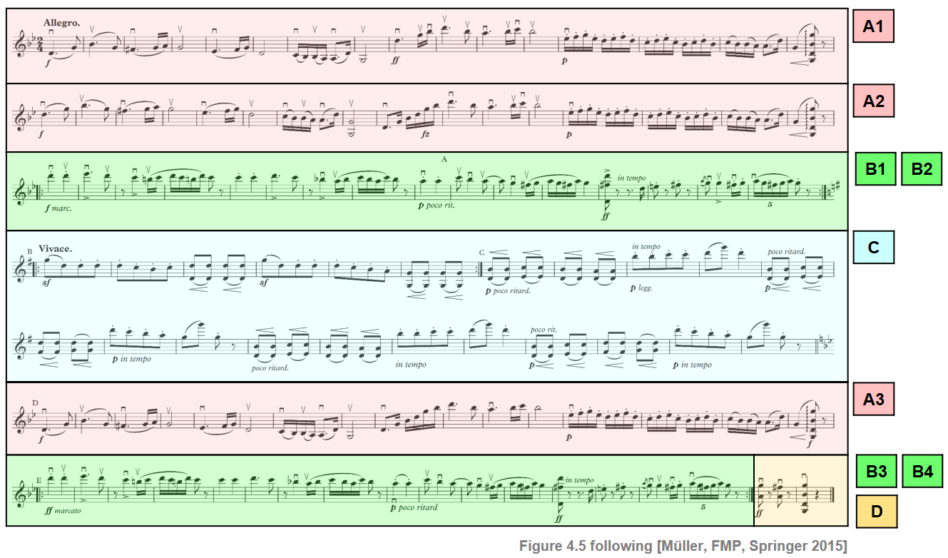
- 음악적 구조는 \(A_1A_2B_1B_2CA_3B_3B_4D\)로 \(A\) 파트 3개, \(B\) 파트 4개, \(C\) 파트 1개, 닫는 \(D\) 파트 1개로 구성되어 있다. \(A\) 부분에는 두 개 이상 반복되는 하위 부분으로 구성된 하위 구조가 있다. 또한 악보를 보면 알 수 있듯이 중간 \(C\) 부분은 \(d_1d_2e_1e_2e_3e_4\)로 설명할 수 있는 하위 구조로 더 분할될 수 있다. 악보에서 이러한 하위 부분은 종종 소문자 \(a,b,c,\ldots\)를 사용하여 표시된다.
ipd.Image("../img/5.music_structure_analysis/FMP_C4_F28.png", width=400)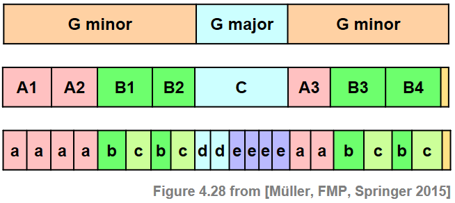
def convert_structure_annotation(ann, Fs=1, remove_digits=False, index=False):
"""Convert structure annotations
Args:
ann (list): Structure annotions
Fs (scalar): Sampling rate (Default value = 1)
remove_digits (bool): Remove digits from labels (Default value = False)
index (bool): Round to nearest integer (Default value = False)
Returns:
ann_converted (list): Converted annotation
"""
ann_converted = []
for r in ann:
s = r[0] * Fs
t = r[1] * Fs
if index:
s = int(np.round(s))
t = int(np.round(t))
if remove_digits:
label = ''.join([i for i in r[2] if not i.isdigit()])
else:
label = r[2]
ann_converted = ann_converted + [[s, t, label]]
return ann_converted
def read_structure_annotation(fn_ann, fn_ann_color, Fs=1, remove_digits=False, index=False):
"""Read and convert structure annotation and colors
Args:
fn_ann (str): Path and filename for structure annotions
fn_ann_color (str): Filename used to identify colors (Default value = '')
Fs (scalar): Sampling rate (Default value = 1)
remove_digits (bool): Remove digits from labels (Default value = False)
index (bool): Round to nearest integer (Default value = False)
Returns:
ann (list): Annotations
color_ann (dict): Color scheme
"""
df = pd.read_csv(fn_ann, sep=';', keep_default_na=False, header=0)
ann = [(start, end, label) for i, (start, end, label) in df.iterrows()]
ann = convert_structure_annotation(ann, Fs=Fs, remove_digits=remove_digits, index=index)
color_ann = {}
if len(fn_ann_color) > 0:
color_ann = fn_ann_color
if remove_digits:
color_ann_reduced = {}
for key, value in color_ann.items():
key_new = ''.join([i for i in key if not i.isdigit()])
color_ann_reduced[key_new] = value
color_ann = color_ann_reduced
return ann, color_annann_color = {'A1': [1, 0, 0, 0.2], 'A2': [1, 0, 0, 0.2], 'A3': [1, 0, 0, 0.2],
'B1': [0, 1, 0, 0.2], 'B2': [0, 1, 0, 0.2], 'B3': [0, 1, 0, 0.2],
'B4': [0, 1, 0, 0.2], 'C': [0, 0, 1, 0.2], '': [1, 1, 1, 0]}# Annotation file
fn_ann = "../data_FMP/FMP_C4_Audio_Brahms_HungarianDances-05_Ormandy.csv"
# Read annotations
ann, color_ann = read_structure_annotation(fn_ann, fn_ann_color=fn_ann_color)
print('Original annotations with time specified in seconds')
print('Annotations:', ann)
print('Colors:', color_ann)
fig, ax = plot_segments(ann, figsize=(8, 1.2), colors=color_ann, time_label='Time (seconds)')
plt.show()
# Read and convert annotations
Fs = 2
ann, color_ann = read_structure_annotation(fn_ann, fn_ann_color=fn_ann_color, Fs=Fs, remove_digits=True, index=True)
print('Converted annotations (Fs = %d) with reduced labels (removing digits)'%Fs)
print('Annotations:', ann)
print('Colors:', color_ann)
fig, ax = plot_segments(ann, figsize=(8, 1.2), colors=color_ann, time_label='Time (frames)')
plt.show()Original annotations with time specified in seconds
Annotations: [[0.0, 1.01, ''], [1.01, 22.11, 'A1'], [22.11, 43.06, 'A2'], [43.06, 69.42, 'B1'], [69.42, 89.57, 'B2'], [89.57, 131.64, 'C'], [131.64, 150.84, 'A3'], [150.84, 176.96, 'B3'], [176.96, 196.9, 'B4'], [196.9, 199.64, '']]
Colors: {'A1': [1, 0, 0, 0.2], 'A2': [1, 0, 0, 0.2], 'A3': [1, 0, 0, 0.2], 'B1': [0, 1, 0, 0.2], 'B2': [0, 1, 0, 0.2], 'B3': [0, 1, 0, 0.2], 'B4': [0, 1, 0, 0.2], 'C': [0, 0, 1, 0.2], '': [1, 1, 1, 0]}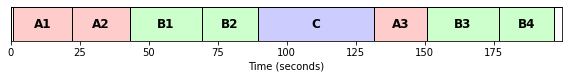
Converted annotations (Fs = 2) with reduced labels (removing digits)
Annotations: [[0, 2, ''], [2, 44, 'A'], [44, 86, 'A'], [86, 139, 'B'], [139, 179, 'B'], [179, 263, 'C'], [263, 302, 'A'], [302, 354, 'B'], [354, 394, 'B'], [394, 399, '']]
Colors: {'A': [1, 0, 0, 0.2], 'B': [0, 1, 0, 0.2], 'C': [0, 0, 1, 0.2], '': [1, 1, 1, 0]}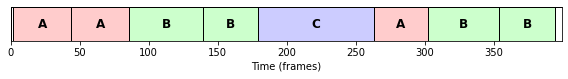
음악적 차원의 분할
- 다양한 분할 원리(segmentation principle)의 적용 가능성은 분석할 오디오 신호의 음악적 및 음향적 특성에 크게 좌우된다. 예를 들어, 구조적 경계(bounadary)는 화음, 음색 또는 템포의 변화를 기반으로 할 수 있다.
- 구조 분석의 첫 번째 단계는 주어진 음악 녹음을 관련 음악 속성을 캡처하는 적절한 특징 표현으로 변환하는 것이다. 다음에서는 세 가지 다른 유형의 특징(feature) 표현(크로마그램, MFFC, 템포그램)을 살펴본다.
- 또한 하나의 특징 유형의 경우에도 특징 표현 품질에 상당한 영향을 미치는 많은 변형과 다양한 매개변수 설정이 있다.
fn_wav = '../data_FMP/FMP_C4_Audio_Brahms_HungarianDances-05_Ormandy.wav'
x, Fs = librosa.load(fn_wav)
ipd.Audio(x,rate=Fs)