머신러닝을 이용한 트레이딩: (3) 피쳐 생성

Get Market Features

trading

feature

momentum

Author

Cheonghyo Cho

앞서 구한 시장 데이터를 이용하여 피쳐(feature)를 생성한다.

피쳐의 종류는 아래에서 설명한다.

# lib
import numpy as np
import pandas as pd
import matplotlib.pyplot as plt
import seaborn as sns;sns.set()
plt.style.use('tableau-colorblind10')

# homemade
from features import tautil, sadf, trnd_scan, microstructure_features

시장 데이터

mtd_data = pd.read_excel('C:data/mtd_data.xlsx')
date = mtd_data.iloc[:,1].rename('Date')
open = mtd_data.iloc[:,2].rename('open')
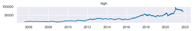
high = mtd_data.iloc[:,3].rename('high')
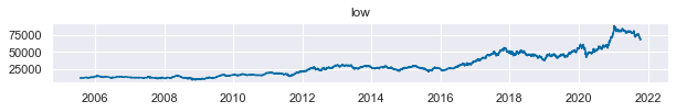
low = mtd_data.iloc[:,4].rename('low')
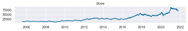
close = mtd_data.iloc[:,5].rename('close')
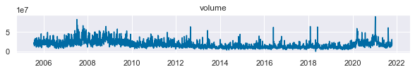
volume = mtd_data.iloc[:,6].rename('volume')

df = pd.DataFrame([open,high,low,close,volume]).T
df.index=date

quantity_ = pd.read_csv('C:data/순매수량.csv')
quantity_ = quantity_.iloc[:-1,1:5]
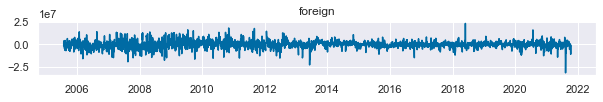
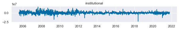
quantity_.columns = ['Date','individual','foreign','institutional']
quantity_.index = quantity_['Date'].apply(lambda x: pd.to_datetime(str(x), format='%Y%m%d'))
quantity_.drop(columns='Date',inplace=True)
df = df.join(quantity_).dropna()

df.to_csv("C:data/market_samsung.csv")
df

	open	high	low	close	volume	individual	foreign	institutional
Date
2005-07-27	11040	11180	10960	11020	18434300	-2543250.0	-1411300.0	-1210850.0
2005-07-28	11040	11320	11040	11200	23659800	-2067600.0	3772300.0	-1517250.0
2005-07-29	11320	11320	11200	11300	17875500	1583050.0	796450.0	-1843600.0
2005-08-01	11320	11380	11220	11380	16471100	-3111550.0	1520100.0	-2652100.0
2005-08-02	11400	11420	11240	11360	14254000	-1567950.0	-1895300.0	-1310950.0
...	...	...	...	...	...	...	...	...
2021-10-08	72300	72400	71500	71500	14043287	2612855.0	319900.0	-2923031.0
2021-10-12	70700	70900	68700	69000	31001484	12155071.0	-11004329.0	-1421202.0
2021-10-13	68700	69600	68300	68800	24172015	2224620.0	-5271845.0	2725596.0
2021-10-14	69000	69800	68800	69400	19520641	2011163.0	-3787173.0	1696662.0
2021-10-15	70200	71000	70000	70100	18051612	822742.0	-1376104.0	456288.0

3965 rows × 8 columns

for i in df.columns:
    plt.figure(figsize=(10,1))
    plt.title(i)
    plt.plot(df[i])

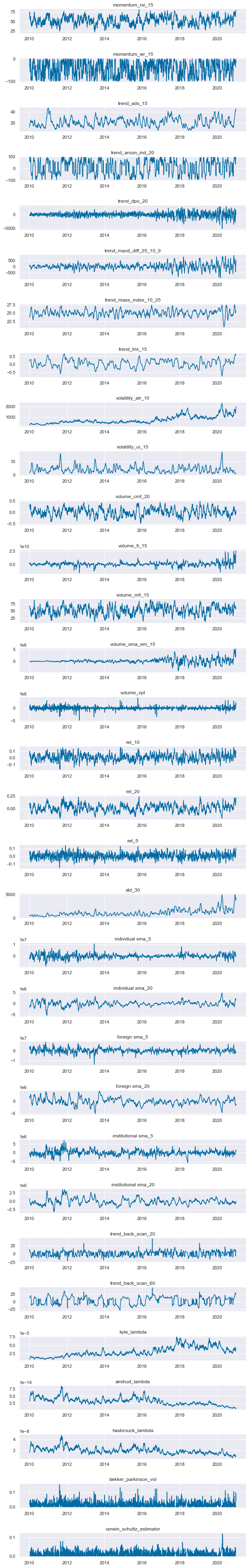
피쳐 변수 (Feature)

14개의 기술적분석 지표 (괄호안 숫자는 각 지표를 구하기 위한 window)
- RSI (15)
- Willams’s R (15)
- ADX (15)
- AROON Indicator (20)
- DPO (20)
- MACD Difference (25,10,9)
- Mass Index (10, 25)
- TRIX (15)
- ATR (10)
- UI (15)
- CMF (20)
- FI (15)
- MFI (15)
- EOM SMA (15)
- VPT
5,10,20일 기간의 가격 수익률
30일 기간의 가격 변동성(표준편차)
개인, 기관, 외국인 별 순매수량의 5일, 20일
트렌드-스캐닝 백워드 t value span (20,60)
미시구조론 변수 각 20일 이동평균
- kyle_lambda
- amihud_lambda
- hasbrouck_lambda
- bekker_parkinson_volatility
- corwin_schultz_estimator

windows_TA = [1]
TA = tautil.get_my_stationary_ta_windows(df_ohlcv,windows_TA).dropna()

windows_mom = [5,10,20]
windows_std = [30]

moms = tautil.mom_std(df,windows_mom, windows_std)
moms = moms.iloc[:,:len(windows_mom)+len(windows_std)]

quantity_ = pd.read_csv('C:data/순매수량.csv')
quantity_ = quantity_.iloc[:-1,1:5]
quantity_.columns = ['Date','individual','foreign','institutional']
quantity_.index = quantity_['Date'].apply(lambda x: pd.to_datetime(str(x), format='%Y%m%d'))
quantity_.drop(columns='Date',inplace=True)

windows_ma=[5,20]
for i in quantity_.columns:
    for j in windows_ma:
        quantity_['{} sma_{}'.format(i,j)] = quantity_[i].rolling(j).mean()
        quantity_.dropna(inplace=True)
quantity = quantity_.iloc[:,3:]

spans = [20,60]
trnd_back = pd.DataFrame()
for span in spans:
    trnd_back['trend_back_scan_{}'.format(span)] = trnd_scan.trend_backward_scanning(df.close, span).t_value

dollar_volume = df.volume*df.close

close=df.close
kyle = microstructure_features.get_bar_based_kyle_lambda(close, df.volume, 20).rename('kyle_lambda')
amihud = microstructure_features.get_bar_based_amihud_lambda(close, dollar_volume, 20).rename('amihud_lambda')
hasbrouk = microstructure_features.get_bar_based_hasbrouck_lambda(close, dollar_volume,20).rename('hasbrouck_lambda')
bp_vol = microstructure_features.get_bekker_parkinson_vol(df.high,df.low,20).rename('bekker_parkinson_vol')
corsch = microstructure_features.get_corwin_schultz_estimator(df.high,df.low,20).rename('corwin_schultz_estimator')

microstructure = pd.concat([kyle,amihud,hasbrouk,bp_vol,corsch],axis=1)

features = TA.join([moms,quantity,trnd_back,microstructure]).dropna()
features.to_csv('C:data/features_samsung.csv')

features = features['2010':'2020']
f, axs = plt.subplots(len(features.T),figsize=(10,70),gridspec_kw={'hspace': 1})
for i in range(len(features.T)):
    axs[i].title.set_text(features.columns[i])
    axs[i].plot(features.iloc[:,i])
f.savefig('C:image/features.png')