\(\mathbf{H}_t\)는 관측 행렬로, 상태 변수가 관측 데이터에 어떻게 영향을 미치는지 설명한다.
\(\mathbf{v}_t\)는 관측 노이즈로, 관측 과정에서 발생하는 오차를 나타낸다.
Kalman Filter
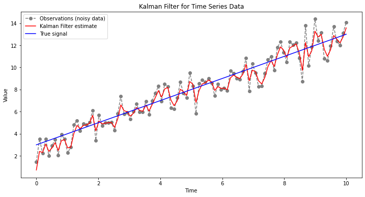
칼만 필터(Kalman filter)는 선형 동적 시스템에서 시간에 따라 변하는 신호를 최적으로 추정하기 위해 사용되는 재귀적 알고리즘이다. 특히 잡음이 있는 데이터를 처리할 때 유용하다. 칼만 필터는 과거에 수행한 측정값을 바탕으로 현재의 상태 변수의 결합분포를 추정한다. 알고리즘은 예측과 업데이트의 두 단계로 이루어진다.
<예측 단계>
현재의 상태 추정치와 공분산을 기반으로 다음 시간 단계의 상태 추정치와 공분산을 예측한다.
상태예측: - \(\hat{x}_{k|k-1} = F_k \hat{x}_{k-1|k-1} + B_k u_k\) - \(\hat{x}_{k|k-1}\)는 시간 \(k\)에서의 상태 예측값, \(F_k\)는 상태 전이 행렬, \(\hat{x}_{k-1|k-1}\)는 이전 시간 \(k-1\)에서의 상태 추정치, \(B_k\)는 제어 입력 행렬, \(u_k\)는 제어 입력
상태 업데이트: - \(\hat{x}_{k|k} = \hat{x}_{k|k-1} + K_k (z_k - H_k \hat{x}_{k|k-1})\) - \(z_k\)는 시간 \(k\)에서의 실제 측정값
공분산 업데이트: - \(P_{k|k} = (I - K_k H_k) P_{k|k-1}\)
import numpy as npimport matplotlib.pyplot as pltfrom pykalman import KalmanFilter# 인위적 데이터 생성: 선형 추세 + 잡음n_timesteps =100x = np.linspace(0, 10, n_timesteps)true_signal = x +3observations = true_signal + np.random.normal(0, 1, n_timesteps)# 칼만 필터 설정kf = KalmanFilter(initial_state_mean=0, n_dim_obs=1)# 칼만 필터로 신호 추정state_means, state_covariances = kf.filter(observations)# 결과 시각화plt.figure(figsize=(12, 6))plt.plot(x, observations, label='Observations (noisy data)', linestyle='dashed', marker='o', color='gray')plt.plot(x, state_means, label='Kalman Filter estimate', color='red')plt.plot(x, true_signal, label='True signal', color='blue')plt.legend()plt.title('Kalman Filter for Time Series Data')plt.xlabel('Time')plt.ylabel('Value')plt.show()
칼만 필터의 단점
칼만 필터는 기본적으로 시스템이 선형이고, 잡음이 정규 분포를 따른다고 가정: 아닌 경우 Extended Kalman Filter나 Unscented Kalman Filter와 같은 변형이 필요
초기 상태 추정치나 모델 파라미터(예: 전이 행렬)의 정확도가 부족하면 추정의 정확성이 저하
(계산 복잡성) 칼만 필터는 매 시간 단계마다 행렬 연산을 수행해야 하므로, 행렬의 크기가 크거나 시스템이 복잡해질 경우 계산 비용이 증가할 수 있습니다.
칼만 필터를 적용하기 위해서는 시스템의 동적 모델을 알아야 함
Unscented Kalman Filter
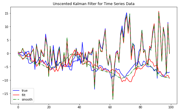
무향 칼만 필터(UKF)는 칼만 필터의 비선형 확장이다.
시스템의 비선형성을 처리하기 위해 ’시그마 포인트’라는 개념을 도입한다. 이는 상태 추정치의 평균과 공분산을 기반으로 선택된 몇 개의 표본 점을 사용하여, 비선형 변환을 통해 이 포인트들을 전파시키는 방식으로 작동한다. 이렇게 전파된 포인트들을 사용하여 업데이트된 평균과 공분산을 계산함으로써 비선형 시스템의 상태를 추정한다.
시그마 포인트 생성: 상태 추정치의 평균과 공분산으로부터 시그마 포인트를 계산
시그마 포인트의 전파: 각 시그마 포인트를 시스템의 비선형 모델을 통해 전파
평균과 공분산 업데이트: 전파된 시그마 포인트들로부터 새로운 평균과 공분산을 계산
측정 업데이트: 새로운 측정값을 사용하여 상태 추정치와 공분산을 업데이트
from pykalman import UnscentedKalmanFilter# initialize parametersdef transition_function(state, noise): a = np.sin(state[0]) + state[1] * noise[0] b = state[1] + noise[1]return np.array([a, b])def observation_function(state, noise): C = np.array([[-1, 0.5], [0.2, 0.1]])return np.dot(C, state) + noisetransition_covariance = np.eye(2)random_state = np.random.RandomState(123)observation_covariance = np.eye(2) + random_state.randn(2, 2) *0.1initial_state_mean = [0, 0]initial_state_covariance = [[1, 0.1], [-0.1, 1]]# sample from modelkf = UnscentedKalmanFilter( transition_function, observation_function, transition_covariance, observation_covariance, initial_state_mean, initial_state_covariance, random_state=random_state)states, observations = kf.sample(100, initial_state_mean)# estimate state with filtering and smoothingfiltered_state_estimates = kf.filter(observations)[0]smoothed_state_estimates = kf.smooth(observations)[0]# draw estimatesplt.figure(figsize=(10,6))plt.title('Unscented Kalman Filter for Time Series Data')lines_true = plt.plot(states, color='b')lines_filt = plt.plot(filtered_state_estimates, color='r', ls='-')lines_smooth = plt.plot(smoothed_state_estimates, color='g', ls='-.')plt.legend((lines_true[0], lines_filt[0], lines_smooth[0]), ('true', 'filt', 'smooth'), loc='lower left')plt.show()
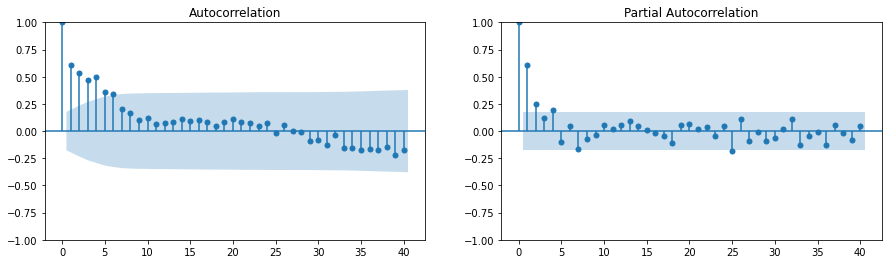
AR (AutoRegressive) 부분: 과거의 종속 변수 값(지연 값)이 미래 값에 영향을 미친다고 가정
MA (Moving Average) 부분: 과거의 예측 오차가 미래 예측에 영향을 미친다고 가정
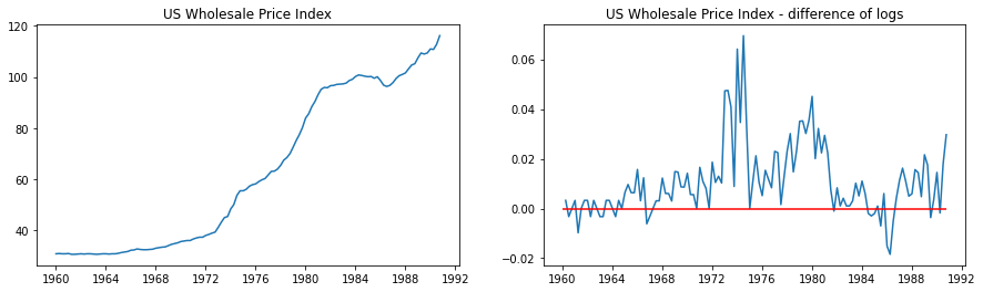
Integration (차분) 부분: 비정상성(Non-stationarity) 데이터를 정상성(Stationarity) 데이터로 변환하기 위해 사용
Seasonal 요소: 계절성 패턴을 모델링. 계절성 AR 및 MA 구성 요소와 계절성 차분 차수를 포함할 수 있으며, 이들은 각각 \(P, D, Q\) 및 계절 주기 \(s\)에 의해 정의됨
Exogenous 변수 (\(\mathbf{X}\)): 모델에 외부에서 영향을 미치는 변수(예: 경제 지표, 마케팅 캠페인, 기상 조건 등)를 포함. 이 변수들은 종속 변수에 직접적인 영향을 미칠 수 있으며, 모델의 설명력과 예측력을 향상시킴.
import numpy as npimport pandas as pdfrom scipy.stats import normimport statsmodels.api as smimport matplotlib.pyplot as pltfrom datetime import datetime
data = pd.read_stata('data/wpi1.dta')data.index = data.t# Set the frequencydata.index.freq="QS-OCT"data['ln_wpi'] = np.log(data['wpi'])data['D.ln_wpi'] = data['ln_wpi'].diff()# Graph datafig, axes = plt.subplots(1, 2, figsize=(15,4))# Levelsaxes[0].plot(data.index._mpl_repr(), data['wpi'], '-')axes[0].set(title='US Wholesale Price Index')# Log differenceaxes[1].plot(data.index._mpl_repr(), data['D.ln_wpi'], '-')axes[1].hlines(0, data.index[0], data.index[-1], 'r')axes[1].set(title='US Wholesale Price Index - difference of logs');
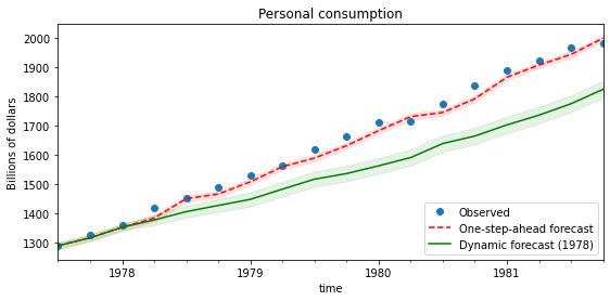
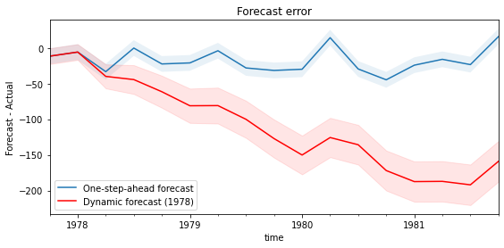
# get results for the full dataset but using the estimated parameters (on a subset of the data)mod = sm.tsa.statespace.SARIMAX(endog, exog=exog, order=(1,0,1))res = mod.filter(fit_res.params)
은닉 마르코프 모델(Hidden Markov Model, HMM)은 시간에 따라 변하는 시스템의 상태를 모델링하기 위한 통계적 모델이다. 이 모델은 관측할 수 없는(은닉된) 상태가 시간에 따라 마르코프 과정(Markov process)에 따라 변화하며, 각 상태는 특정 확률 분포를 가지고 관측 가능한 결과를 생성한다고 가정한다. HMM은 이러한 은닉 상태와 관측된 데이터 사이의 관계를 모델링하는 데 사용된다.
HMM의 구성 요소
상태(state): 모델의 각 상태는 시스템이 취할 수 있는 잠재적 상태를 나타내며, 이 상태들은 직접 관찰할 수 없음.
은닉 상태 \(S=\{s_1,s_2, \dots, s_N \}\)
관찰(observation): 각 상태에서 특정 관찰이 나타날 확률을 나타내며, 이 관찰은 실제로 측정되거나 관찰할 수 있는 데이터 포인트
관찰 \(O = \{o_1,o_2,\dots,o_T\}\)
전이 확률(transition probabilities): 한 상태(\(s_i\))에서 다음 상태(\(s_j\))로 이동할 확률
\(a_{ij}=P(q_{t+1}=s_j|q_t=s_i)\)
발생 확률(emission probabilities): 각 상태(\(s_i\))에서 특정 관찰(\(o_k\))이 발생할 확률
\(b_{ik}=P(o_t=v_k|q_t=s_i)\)
초기 상태 확률(initial state probabilities) \(\pi\): 시퀀스의 시작에서 각 상태가 초기 상태(\(s_i\))일 확률
\(\pi_i = P(q_1=s_i)\)
확률 계산(Forward 알고리즘)
주어진 모델 \(\lambda = (A,B,\pi)\)과 관찰 시퀀스 \(O\)에 대해, \(P(O|\lambda)\)를 계산한다. 이는 Forward 알고리즘을 사용해 해결할 수 있다.
Forward 변수 : \(\alpha_t(i)\) 시간 \(t\)에서 상태 \(i\)에 있을 확률, 관찰 \(O\)가 주어졌을 때의 확률을 의미한다. \[\alpha_t(j) = \left(\sum_{i=1}^N \alpha_{t-1}(i) a_{ij}\right) b_j(o_t)\]
주어진 관찰 시퀀스와 모델에 대해 가장 가능성 높은 은닉 상태 시퀀스를 찾는다.(decoding) 이는 Viterbi 알고리즘을 사용하여 해결할 수 있다.
Viterbi 변수: 최적 경로의 확률로, 시간 \(t\)에서 상태 \(i\)에 도달하기까지의 최대 확률을 의미한다. \[\delta_t(j) = \max_{1 \leq i \leq N} (\delta_{t-1}(i) a_{ij}) b_j(o_t)\]
초기화: \[\delta_1(i) = \pi_i b_i(o_1)\]
종료: \[P^* = \max_{1 \leq i \leq N} \delta_T(i)\]
모델 학습 (Baum-Welch 알고리즘)
주어진 관찰 시퀀스를 가장 잘 설명할 수 있는 모델 매개변수를 추정한다. Baum-Welch 알고리즘(EM 알고리즘의 한 형태)을 사용하여 반복적으로 매개변수를 최적화한다.
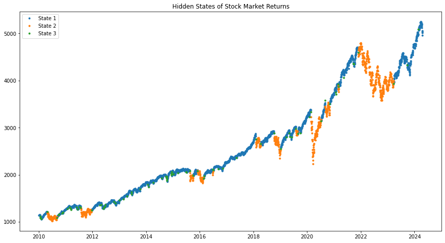
import numpy as npimport pandas as pdimport matplotlib.pyplot as pltimport yfinance as yffrom hmmlearn.hmm import GaussianHMMdata = yf.download('^GSPC', '2010-01-01')data = data['Close']log_returns = np.log(data / data.shift(1))[1:] # 로그 수익률 계산log_returns = log_returns.values.reshape(-1, 1) # HMM 입력 형태 맞추기
[*********************100%%**********************] 1 of 1 completed
# HMM 모델 초기화 (은닉 상태의 수: 3)hmm_model = GaussianHMM(n_components=3, covariance_type="diag", n_iter=1000)hmm_model.fit(log_returns) # 모델 학습# 은닉 상태 예측hidden_states = hmm_model.predict(log_returns)## hidden_states = hmm_model.decode(log_returns)[1]
Model is not converging. Current: 11839.472901701653 is not greater than 11839.483144542859. Delta is -0.010242841206490993
# 결과 시각화plt.figure(figsize=(15, 8))data_t = data[1:]for i inrange(hmm_model.n_components): state = (hidden_states == i) plt.plot(data_t.index[state], data_t[state], '.', label=f'State {i+1}')plt.legend()plt.title('Hidden States of Stock Market Returns')plt.show()